Thermal Performances of Windows

During the design of a building, environmental issues have gained considerable influence in the entire project. One of the first concerns is to improve thermal performances. In this process, simulation software provide key tools for modeling thermal losses and performances in the building.

The international standard ISO 10077-2:2012 (Ref. 1) deals with thermal performances of windows, doors, and shutters. It provides computed values of the thermal characteristics of frame profiles in order to validate a simulation software.

COMSOL Multiphysics successfully passes the entire benchmark. This document describes six frame profiles of ISO 10077-2:2012 related to windows only. Other test cases from this standard are available in the following applications:

•

Thermal Performances of Roller Shutters

•

Glazing Influence on Thermal Performances of a Window

Figure 1: Geometry of one of the windows and cross-section view.

Model Definition

On each test case, a window section separates a hot internal side from a cold external side. In these applications, the traditional glazing is replaced by an insulation panel. After solving a model, two quantities are calculated and compared to the normative values:

•

The thermal conductance between the internal and external sides

•

The thermal transmittance of the window frame

air cavities

A window frame contains many cavities. The purpose is to ensure thermal insulation. According to the standard, cavities are modeled in different ways depending on their shapes.

The heat flow rate in cavities is represented by an equivalent thermal conductivity keq, which includes the heat flow by conduction, convection, and radiation. It also depends on the geometry of the cavity and on the adjacent materials. The definition of keq is detailed in the next paragraphs.

Cavities are divided into three types:

•

unventilated cavities, completely closed or connected either to the exterior or to the interior by a slit with a width not exceeding 2 mm;

•

slightly ventilated cavities, connected either to the exterior or to the interior by a slit greater than 2 mm but not exceeding 10 mm;

•

well-ventilated cavities, corresponding to a configuration not covered by one of the two preceding types, it is assumed that the whole surface is exposed to the environment so that boundary conditions are applied to (see the Boundary conditions section below for more information).

Unventilated Rectangular Cavity

For an unventilated rectangular cavity, the equivalent thermal conductivity is defined by:

where d is the cavity dimension in the heat flow rate direction, and R is the cavity thermal resistance given by:

where ha is the convective heat transfer coefficient, and hr is the radiative heat transfer coefficient. These coefficients are defined by:

where:

•

C1 = 0.025 W/(m·K)

•

C2 = 0.73 W/(m2·K4/3)

•

ΔT is the maximum surface temperature difference in the cavity

•

σ = 5.67·10-8 W/(m2·K4) is the Stefan-Boltzmann constant

•

Tm is the average temperature on the boundaries of the cavity

•

E is the intersurface emittance, defined by:

•

ε1 and ε2 are the surface emissivities (both are equal to 0.90 in this model)

•

F is the view factor of the rectangular section, defined by:

•

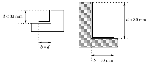
d is the cavity dimension in the heat flow rate direction

•

b is the cavity dimension perpendicular to the heat flow rate direction

Slightly Ventilated Rectangular Cavities

For a slightly ventilated cavity, the equivalent thermal conductivity is twice that of an unventilated cavity of the same size.

Nonrectangular Cavities

Nonrectangular cavities are transformed into rectangular cavities of same area and aspect ratio according to defined rules in ISO 10077-2:2012 presented below. Then, keq is evaluated following one of the two previous rectangular cases.

Figure 2: Nonrectangular cavity transformation.

Figure 2 shows a nonrectangular cavity of area A′. Then, d′ and b′ are the depth and the width (in accordance with the direction of the heat flow) of the smallest rectangle than can contain of the nonrectangular cavity. The equivalent rectangular cavity, of size b × d and area A must satisfy:

Hence, b and d are given by:

Boundary conditions

The heat flux conditions for internal and external sides are given by Newton’s law of cooling:

where Text is the exterior temperature (Text = Ti = 20°C for the internal side and Text = Te = 0°C for the external side). The standard defines thermal surface resistance, Rs, which is related to the heat transfer coefficient, h, by:

Internal and external thermal surface resistances are not equal. Moreover, on boundaries linked to the internal side, an increased thermal resistance is used in edges. Figure 3 explains how to determine boundaries where it should be applied.

Figure 3: Protected boundaries.

If d is greater than 30 mm, b is set to 30 mm. Otherwise, b = d is chosen. Furthermore, two boundaries are considered as adiabatic: the boundary in contact with the wall and the end of the insulation panel.

Description of the six Applications

Figure 4 to Figure 9 depict the geometry of each application but only a part of the insulation panel is represented. Unventilated cavities are red-numbered while slightly ventilated cavities are green-numbered. Boundaries with an increased thermal resistance are represented with bold black lines. Adiabatic boundaries in contact with the wall are represented with a striped rectangle.

Application 1: Aluminum Frame with Thermal Break

The first application studies the heat conduction in an aluminum frame section with thermal break. The frame structure is made of aluminum with a high thermal conductivity k of 160 W/(m·K). Four barriers made of polyamide 6.6 with 25% of glass fiber compose the thermal break. They have a low thermal conductivity of 0.30 W/(m·K). Ethylene propylene diene monomer (EPDM) rubber gaskets are also used to waterproof the window. EPDM rubber has a thermal conductivity of 0.25 W/(m·K). The insulation panel has a very low thermal conductivity of 0.035 W/(m·K).

This frame is divided into many cavities: most of them are considered as unventilated cavities because they are not connected to the exterior. One cavity is connected to the exterior. According to the standard, this cavity is cut into two “subcavities” due to its internal 2 mm width slit. The first cavity (labeled 1 on Figure 4) is considered as unventilated cavity and the second cavity (labeled 10 on Figure 4) are considered as a slightly ventilated cavity.

Figure 4: Geometry of the first window.

Application 2: Aluminum Clad Wood Frame

The second application studies the heat conduction in an aluminum clad wood frame section. The frame is made of two wood blocks with a thermal conductivity of 0.13 W/(m·K). On the external side, a wood block is covered by an aluminum structure which has a high thermal conductivity. This application includes EPDM gaskets too.

All cavities is considered as an unventilated cavities because they are either closed or connected to the exterior by a 2 mm width slit.

Figure 5: Geometry of the second window.

Application 3: PVC Frame with Steel Reinforcement

The third application studies the heat conduction in a PVC frame section with steel reinforcement. The main structure of the frame is made of PVC, which has a thermal conductivity of 0.17 W/(m·K). Two reinforcements made of steel are also present. Steel has a high thermal conductivity of 50 W/(m·K). EPDM gaskets are used.

Air cavities are all completely closed or connected to the exterior by a slit with a width not exceeding 2 mm. Thus they are considered as unventilated cavities.

Figure 6: Geometry of the third window.

Application 4: Roof Window

The fourth application studies the heat conduction in a roof window frame section. The main part of the frame is made of two soft wood blocks. The interior part is aluminum clad and there are also EPDM gaskets.

Three air cavities are not connected to the exterior or only by a slit with a width smaller than 2 mm. They are considered as unventilated. Four others air cavities are considered as slightly ventilated cavities.

Figure 7: Geometry of the fourth window.

Application 5: Sliding Window

The fifth application studies the heat conduction in a sliding window frame section. The frame has an aluminum structure with a high thermal conductivity. There are some thermal breaks made of rigid polyurethane (PU), polyamide, and polyester mohair. Their thermal conductivities are 0.25 W/(m·K), 0.25 W/(m·K), and 0.14 W/(m·K), respectively. There are also some EPDM gaskets to waterproof the window.

Four air cavities are completely closed, and two others are connected to the exterior by a 2 mm width slit. According to the standard, they are considered as unventilated cavities. One cavity is considered as a slightly ventilated cavity because it is connected to the exterior by a larger slit of 6 mm. In addition, one last cavity is considered as well ventilated because it is connected to the exterior with a 15 mm width slit.

Figure 8: Geometry of the fifth window.

Application 6: PVC Frame

The sixth application studies the heat conduction in a fixed PVC frame section. Polyamide with a thermal conductivity of 0.25 W/(m·K) is used. There are also some EPDM gaskets to waterproof the window.

In this application, there are seven closed cavities. There are considered as unventilated. In addition, one cavity is connected to the exterior by a 3 mm width slit so it is considered as slightly ventilated.

Figure 9: Geometry of the sixth window.

Results and Discussion

Temperature profiles

The temperature profiles for each application are shown in Figure 10 to Figure 15.

Figure 10: Temperature distribution in the aluminum frame with thermal break.

Figure 11: Temperature distribution in the aluminum clad wood frame.

Figure 12: Temperature distribution in the PVC frame with steel reinforcement.

Figure 13: Temperature distribution in the roof window.

Figure 14: Temperature distribution in the sliding window.

Figure 15: Temperature distribution in the PVC frame.

Quantities of interest

The quantities of interest are the following:

•

The thermal conductance of the entire section L2D given by:

where

is the heat flow rate through the window (in W/m), Te = 0°C is the external temperature and Ti = 20°C is the internal temperature

•

The thermal transmittance of the frame Uf defined by:

where bp is the visible width of the panel expressed in meters, bf is the projected width of the frame section expressed in meters, and Up is the thermal transmittance of the central area of the panel expressed in W/(m2·K).

Table 1 to Table 6 compare the numerical results of COMSOL Multiphysics with the expected values provided by ISO 10077-2:2012.

Table 1: comparison between expected and computed values of quantities in Application 1.


Quantity	Expected value	Computed Value	Relative Error
L2D (W/(m·K))	0.550	0.556	1.09%
Uf (W/(m2·K))	3.22	3.29	2.13%

Table 2: comparison between expected and computed values of quantities in Application 2.


Quantity	Expected value	Computed Value	Relative Error
L2D (W/(m·K))	0.263	0.265	0.76%
Uf (W/(m2·K))	1.44	1.466	1.8%

Table 3: comparison between expected and computed values of quantities in Application 3.


L2D (W/(m·K))	Expected value	Computed Value	Relative Error
L2D (W/(m·K))	0.424	0.428	0.94%
Uf (W/(m2·K))	2.07	2.12	2.42%

Table 4: comparison between expected and computed values of quantities in Application 4.


L2D (W/(m·K))	Expected value	Computed Value	Relative Error
L2D (W/(m·K))	0.408	0.41	0.49%
Uf (W/(m2·K))	2.08	2.14	2.88%

Table 5: comparison between expected and computed values of quantities in Application 5.


L2D (W/(m·K))	Expected value	Computed Value	Relative Error
L2D (W/(m·K))	0.659	0.656	0.46%
Uf (W/(m2·K))	4.67	4.64	0.64%

Table 6: comparison between expected and computed values of quantities in Application 6.


L2D (W/(m·K))	Expected value	Computed Value	Relative Error
L2D (W/(m·K))	0.285	0.284	0.35%
Uf (W/(m2·K))	1.31	1.346	2.75%

The maximum permissible differences to pass this test case are 3% for the thermal conductance and 5% for the thermal transmittance. The measured values are completely coherent and meet the validation criteria.

Reference

1. European Committee for Standardization, ISO 10077-2:2012, Thermal performance of windows, doors and shutters – Calculation of thermal transmittance – Part 2: Numerical method for frames, 2012.

Heat_Transfer_Module/Buildings_and_Constructions/windows_thermal_performances

Modeling Instructions

Root

Start by opening the following prepared file. It already contains global definitions, geometries, local variables, selections, operators and material properties.

From the menu, choose .

Browse to the model’s Application Libraries folder and double-click the file windows_thermal_performances_preset.mph.

First Window (comp1)

Click the