PDF

Heat Sink with Surface-to-Surface Radiation
Introduction
This application extends the Heat Sink model by taking surface-to-surface radiation into account. For a detailed description of the application, see Heat Sink.
Application Library path: Heat_Transfer_Module/Tutorials,_Forced_and_Natural_Convection/heat_sink_surface_radiation
Modeling Instructions
Root
In this second part you modify and solve the model to study the effects of surface-to-surface radiation between the heat sink and the channel walls.
1
From the File menu, choose Open.
2
Component 1 (comp1)
Now modify the model to include surface-to-surface radiation effects. First you need to enable the surface-to-surface radiation property.
Heat Transfer in Solids and Fluids (ht)
By default, the radiation direction is controlled by the opacity of the domains. The solid parts are automatically defined as opaque while the fluid parts are transparent. You can change these settings by modifying the Opacity subnode under Solid and Fluid features.
When the Diffuse Surface boundary condition defines the radiation direction as opacity controlled (default) the selected boundaries should be located between an opaque and a transparent domain. The exterior is defined as transparent by default. Change this setting to make the exterior opaque and have the radiation direction automatically defined on the channel walls.
Add Physics
1
In the Home toolbar, click  Add Physics to open the Add Physics window.
2
Go to the Add Physics window.
3
In the tree, select Heat Transfer>Radiation>Surface-to-Surface Radiation (rad).
4
Click Add to Component 1 in the window toolbar.
5
In the Home toolbar, click  Add Physics to close the Add Physics window.
Surface-to-Surface Radiation (rad)
Now you can add a surface-to-surface boundary condition to the model.
1
In the Settings window for Surface-to-Surface Radiation, locate the Boundary Selection section.
2
From the Selection list, choose Exterior Walls.
Diffuse Surface 1
1
In the Model Builder window, under Component 1 (comp1)>Surface-to-Surface Radiation (rad) click Diffuse Surface 1.
2
In the Settings window for Diffuse Surface, locate the Ambient section.
3
Find the Ambient temperature subsection. From the Tamb list, choose Ambient temperature (ampr1).
4
Locate the Surface Emissivity section. From the ε list, choose User defined. In the associated text field, type 0.85.
Opacity 1
1
In the Physics toolbar, click  Domains and choose Opacity.
2
In the Settings window for Opacity, locate the Domain Selection section.
3
From the Selection list, choose All voids.
Add Multiphysics
1
In the Physics toolbar, click  Add Multiphysics to open the Add Multiphysics window.
2
Go to the Add Multiphysics window.
3
In the tree, select No Predefined Multiphysics Available for the Selected Physics Interfaces.
4
Find the Select the physics interfaces you want to couple subsection. In the table, clear the Couple check box for Laminar Flow (spf).
5
In the tree, select Heat Transfer>Radiation>Heat Transfer with Surface-to-Surface Radiation.
6
Click Add to Component in the window toolbar.
7
In the Physics toolbar, click  Add Multiphysics to close the Add Multiphysics window.
Component 1 (comp1)
Hide the boundaries on the top and fronts to see the interior of the channel and the heat sink.
1
Click the  Click and Hide button in the Graphics toolbar.
2
Click the  Select Boundaries button in the Graphics toolbar.
3
In the Model Builder window, click Component 1 (comp1).
4
Root
In order to keep the previous solution and to be able to compare it with this version of the model, create a new stationary study.
Add Study
1
In the Home toolbar, click  Add Study to open the Add Study window.
2
Go to the Add Study window.
3
Find the Studies subsection. In the Select Study tree, select General Studies>Stationary.
4
Click Add Study in the window toolbar.
5
In the Home toolbar, click  Add Study to close the Add Study window.
Study 1 - without radiation
1
In the Model Builder window, right-click Study 1 and choose Rename.
2
In the Rename Study dialog box, type Study 1 - without radiation in the New label text field.
3
Study 2 - with radiation
1
In the Model Builder window, right-click Study 2 and choose Rename.
2
In the Rename Study dialog box, type Study 2 - with radiation in the New label text field.
3
4
In the Home toolbar, click  Compute.
Results
Temperature (ht) 1
The same default plots as before are generated automatically. Modify the temperature plot to compare both cases.
Arrow Volume 1
1
In the Temperature (ht) 1 toolbar, click  Arrow Volume.
2
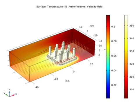
In the Settings window for Arrow Volume, click Replace Expression in the upper-right corner of the Expression section. From the menu, choose Component 1 (comp1)>Laminar Flow>Velocity and pressure>u,v,w - Velocity field.
3
Locate the Data section. From the Dataset list, choose Study 2 - with radiation/Solution 2 (sol2).
4
Locate the Arrow Positioning section. Find the x grid points subsection. In the Points text field, type 40.
5
Find the y grid points subsection. In the Points text field, type 20.
6
Find the z grid points subsection. From the Entry method list, choose Coordinates.
7
In the Coordinates text field, type 5[mm].
Color Expression 1
1
In the Temperature (ht) 1 toolbar, click  Color Expression.
2
In the Settings window for Color Expression, click Replace Expression in the upper-right corner of the Expression section. From the menu, choose Component 1 (comp1)>Laminar Flow>Velocity and pressure>spf.U - Velocity magnitude - m/s.
3
In the Temperature (ht) 1 toolbar, click  Plot.
The plot in the Graphics window should look like that in the figure below.