PDF

Heat Sink
Introduction
This example is intended as a first introduction to simulations of fluid flow and conjugate heat transfer. It shows the following important points:
An extension of the application that takes surface-to-surface radiation into account is also available; see Heat Sink with Surface-to-Surface Radiation.
Figure 1: The application setup including channel and heat sink.
Model Definition
The modeled system consists of an aluminum heat sink for cooling of components in electronic circuits mounted inside a channel of rectangular cross section (see Figure 1).
Such a setup is used to measure the cooling capacity of heat sinks. Air enters the channel at the inlet and exits the channel at the outlet. The base surface of the heat sink receives a 1 W heat flux from an external heat source. All other external faces are thermally insulated.
The cooling capacity of the heat sink can be determined by monitoring the temperature of the base surface of the heat sink.
The model solves a thermal balance for the heat sink and the air flowing in the rectangular channel. Thermal energy is transported through conduction in the aluminum heat sink and through conduction and convection in the cooling air. The temperature field is continuous across the internal surfaces between the heat sink and the air in the channel. The temperature is set at the inlet of the channel. The base of the heat sink receives a 1 W heat flux. The transport of thermal energy at the outlet is dominated by convection.
The flow field is obtained by solving one momentum balance for each space coordinate (x, y, and z) and a mass balance. The inlet velocity is defined by a parabolic velocity profile for fully developed laminar flow. At the outlet, the normal stress is equal the outlet pressure and the tangential stress is canceled. At all solid surfaces, the velocity is set to zero in all three spatial directions.
The thermal conductivity of air, the heat capacity of air, and the air density are all temperature-dependent material properties.
You can find all of the settings mentioned above in the predefined multiphysics coupling for Conjugate Heat Transfer in COMSOL Multiphysics. You also find the material properties, including their temperature dependence, in the Material Browser.
Results
In Figure 2, the hot wake behind the heat sink visible in the plot is a sign of the convective cooling effects. The maximum temperature, reached at the heat sink base, is about 380 K.
Figure 2: The surface plot shows the temperature field on the channel walls and the heat sink surface, while the arrow plot shows the flow velocity field around the heat sink.
Application Library path: Heat_Transfer_Module/Tutorials,_Forced_and_Natural_Convection/heat_sink
Modeling Instructions
From the File menu, choose New.
New
In the New window, click  Model Wizard.
Model Wizard
1
In the Model Wizard window, click  3D.
2
In the Select Physics tree, select Heat Transfer>Conjugate Heat Transfer>Laminar Flow.
3
Click Add.
4
Click  Study.
5
In the Select Study tree, select General Studies>Stationary.
6
Geometry 1
Note that the Geometry representation must be set to COMSOL kernel to fit with the numbering of the boundaries used in these instructions.
The model geometry is available as a parameterized geometry sequence in a separate MPH-file. If you want to create it from scratch yourself, you can follow the instructions in the Geometry Modeling Instructions section. Otherwise, insert the geometry sequence as follows:
1
In the Geometry toolbar, click  Insert Sequence.
2
The application’s Application Library folder is shown in the Application Library path section immediately before the current section. Note that the path given there is relative to the COMSOL Application Library root, which for a standard installation on Windows is C:\Program Files\COMSOL\COMSOL56\Multiphysics\applications.
3
In the Geometry toolbar, click  Build All.
4
Click the  Zoom Extents button in the Graphics toolbar.
To facilitate face selection in the next steps, use the Wireframe rendering option (skip this step if you followed the instructions in the appendix):
5
Click the  Wireframe Rendering button in the Graphics toolbar.
Laminar Flow (spf)
1
In the Model Builder window, under Component 1 (comp1) click Laminar Flow (spf).
2
In the Settings window for Laminar Flow, locate the Domain Selection section.
3
From the Selection list, choose Air.
Heat Transfer in Solids and Fluids (ht)
Fluid 1
1
In the Model Builder window, under Component 1 (comp1)>Heat Transfer in Solids and Fluids (ht) click Fluid 1.
2
In the Settings window for Fluid, locate the Domain Selection section.
3
From the Selection list, choose Air.
Materials
Next, add materials.
Add Material
1
In the Home toolbar, click  Add Material to open the Add Material window.
2
Go to the Add Material window.
3
4
Click Add to Component in the window toolbar.
5
In the tree, select Built-in>Aluminum 3003-H18.
6
Click Add to Component in the window toolbar.
7
In the tree, select Built-in>Silica glass.
8
Click Add to Component in the window toolbar.
9
In the Home toolbar, click  Add Material to close the Add Material window.
Materials
Air (mat1)
1
In the Model Builder window, under Component 1 (comp1)>Materials click Air (mat1).
2
In the Settings window for Material, locate the Geometric Entity Selection section.
3
From the Selection list, choose Air.
Aluminum 3003-H18 (mat2)
1
In the Model Builder window, click Aluminum 3003-H18 (mat2).
2
In the Settings window for Material, locate the Geometric Entity Selection section.
3
From the Selection list, choose Aluminum.
Silica glass (mat3)
1
In the Model Builder window, click Silica glass (mat3).
2
In the Settings window for Material, locate the Geometric Entity Selection section.
3
From the Selection list, choose Silica Glass.
Global Definitions
Parameters 1
1
In the Model Builder window, under Global Definitions click Parameters 1.
2
In the Settings window for Parameters, locate the Parameters section.
3
Now define the physical properties of the model. Start with the fluid domain.
Add a node for the ambient properties in the model. The default temperature value is 293.15 K. It is possible to edit the ambient temperature value or to define it using the meteorological data which gives access to climate data from more than 6,000 stations in the world.
Definitions
Ambient Properties 1 (ampr1)
In the Physics toolbar, click  Shared Properties and choose Ambient Properties.
Laminar Flow (spf)
The no-slip condition is the default boundary condition for the fluid. Define the inlet and outlet conditions as described below.
1
In the Model Builder window, under Component 1 (comp1) click Laminar Flow (spf).
Inlet 1
1
In the Physics toolbar, click  Boundaries and choose Inlet.
2
In the Settings window for Inlet, locate the Boundary Selection section.
3
From the Selection list, choose Inlet.
4
Locate the Boundary Condition section. From the list, choose Fully developed flow.
5
Locate the Fully Developed Flow section. In the Uav text field, type U0.
Outlet 1
1
In the Physics toolbar, click  Boundaries and choose Outlet.
2
Click the  Zoom Extents button in the Graphics toolbar.
3
In the Settings window for Outlet, locate the Boundary Selection section.
4
From the Selection list, choose Outlet.
Heat Transfer in Solids and Fluids (ht)
Thermal insulation is the default boundary condition for the temperature. Define the inlet temperature and the outlet condition as described below.
1
In the Model Builder window, under Component 1 (comp1) click Heat Transfer in Solids and Fluids (ht).
Inflow 1
1
In the Physics toolbar, click  Boundaries and choose Inflow.
2
In the Settings window for Inflow, locate the Boundary Selection section.
3
From the Selection list, choose Inlet.
The ambient temperature is defined in the Ambient Properties node under Shared Properties.
Locate the Upstream Properties section. From the Tustr list, choose Ambient temperature (ampr1).
Outflow 1
1
In the Physics toolbar, click  Boundaries and choose Outflow.
2
In the Settings window for Outflow, locate the Boundary Selection section.
3
From the Selection list, choose Outlet.
Next, use the P0 parameter to define the total heat source in the electronics package.
Heat Source 1
1
In the Physics toolbar, click  Domains and choose Heat Source.
2
In the Settings window for Heat Source, locate the Domain Selection section.
3
From the Selection list, choose Silica Glass.
4
Locate the Heat Source section. Click the Heat rate button.
5
In the P0 text field, type P0.
Mesh 1
1
In the Model Builder window, under Component 1 (comp1) click Mesh 1.
2
In the Settings window for Mesh, locate the Physics-Controlled Mesh section.
3
From the Element size list, choose Coarser.
4
Click  Build All.
To get a better view of the mesh, hide some of the boundaries.
5
Click the  Click and Hide button in the Graphics toolbar.
6
Click the  Select Boundaries button in the Graphics toolbar.
7
The finished mesh should look like that in the figure below.
To achieve more accurate numerical results, this mesh can be refined by choosing another predefined element size. However, doing so requires more computational time and memory.
Study 1
In the Home toolbar, click  Compute.
Results
Temperature (ht)
Four default plots are generated automatically. The first one shows the temperature on the wall boundaries, the third one shows the velocity magnitude on five parallel slices, and the last one shows the pressure field. Add an arrow plot to visualize the velocity field with temperature field.
Arrow Volume 1
1
In the Temperature (ht) toolbar, click  Arrow Volume.
2
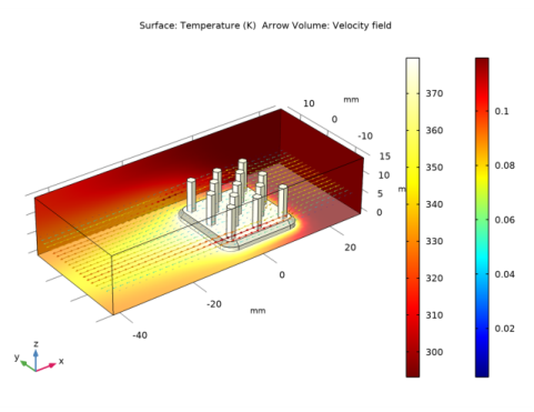
In the Settings window for Arrow Volume, click Replace Expression in the upper-right corner of the Expression section. From the menu, choose Component 1 (comp1)>Laminar Flow>Velocity and pressure>u,v,w - Velocity field.
3
Locate the Arrow Positioning section. Find the x grid points subsection. In the Points text field, type 40.
4
Find the y grid points subsection. In the Points text field, type 20.
5
Find the z grid points subsection. From the Entry method list, choose Coordinates.
6
In the Coordinates text field, type 5[mm].
Color Expression 1
1
In the Temperature (ht) toolbar, click  Color Expression.
2
In the Settings window for Color Expression, click Replace Expression in the upper-right corner of the Expression section. From the menu, choose Component 1 (comp1)>Laminar Flow>Velocity and pressure>spf.U - Velocity magnitude - m/s.
3
In the Temperature (ht) toolbar, click  Plot.
Energy Balance
1
In the Results toolbar, click  Global Evaluation.
2
In the Settings window for Global Evaluation, type Energy Balance in the Label text field.
3
Click Add Expression in the upper-right corner of the Expressions section. From the menu, choose Component 1 (comp1)>Heat Transfer in Solids and Fluids>Heat and energy balance>Energy balance>ht.ntefluxInt - Total net energy rate - W.
4
Click Add Expression in the upper-right corner of the Expressions section. From the menu, choose Component 1 (comp1)>Heat Transfer in Solids and Fluids>Heat and energy balance>Heat and work source powers>ht.QInt - Total heat source - W.
5
Click  Evaluate.
Table
1
Go to the Table window.
You can verify that the two values match and are close to 1 W in the Table 1 tab.
Geometry Modeling Instructions
If you want to create the geometry yourself, follow these steps.
Global Definitions
Parameters 1
1
In the Model Builder window, under Global Definitions click Parameters 1.
2
In the Settings window for Parameters, locate the Parameters section.
3
Add Component
In the Home toolbar, click  Add Component and choose 3D.
Geometry 1
1
In the Settings window for Geometry, locate the Units section.
2
From the Length unit list, choose mm.
Work Plane 1 (wp1)
1
In the Geometry toolbar, click  Work Plane.
2
In the Settings window for Work Plane, locate the Plane Definition section.
3
From the Plane list, choose xz-plane.
4
In the y-coordinate text field, type -7.5.
Work Plane 1 (wp1)>Plane Geometry
In the Model Builder window, click Plane Geometry.
Work Plane 1 (wp1)>Polygon 1 (pol1)
1
In the Work Plane toolbar, click  Polygon.
2
In the Settings window for Polygon, locate the Coordinates section.
3
From the Data source list, choose Vectors.
4
In the xw text field, type -10.495 -9.495 -9.495 -9.495 -9.495 -10.495 -10.495 -10.495.
5
In the yw text field, type 0 0 0 2 2 1 1 0.
Revolve 1 (rev1)
1
In the Model Builder window, under Component 1 (comp1)>Geometry 1 right-click Work Plane 1 (wp1) and choose Revolve.
2
In the Settings window for Revolve, locate the Revolution Angles section.
3
Click the Angles button.
4
In the End angle text field, type 90.
5
Locate the Revolution Axis section. From the Axis type list, choose 3D.
6
Find the Point on the revolution axis subsection. In the x text field, type -7.5.
7
In the y text field, type -7.5.
8
Find the Direction of revolution axis subsection. In the y text field, type 0.
9
In the z text field, type 1.
10
Locate the Selections of Resulting Entities section. Find the Cumulative selection subsection. Click New.
11
In the New Cumulative Selection dialog box, type Aluminum in the Name text field.
12
Extrude 1 (ext1)
1
In the Geometry toolbar, click  Extrude.
2
In the Settings window for Extrude, locate the General section.
3
From the Extrude from list, choose Faces.
4
On the object rev1, select Boundary 1 only.
5
Locate the Distances section. In the table, enter the following settings:
6
Locate the Selections of Resulting Entities section. Find the Cumulative selection subsection. From the Contribute to list, choose Aluminum.
7
Locate the General section. In the tree, select rev1.
Rotate 1 (rot1)
1
In the Geometry toolbar, click  Transforms and choose Rotate.
2
In the Settings window for Rotate, locate the Input section.
3
From the Input objects list, choose Aluminum.
4
Select the Keep input objects check box.
5
Locate the Rotation section. In the Angle text field, type range(90, 90,270).
6
Locate the Selections of Resulting Entities section. Find the Cumulative selection subsection. From the Contribute to list, choose Aluminum.
Work Plane 2 (wp2)
1
In the Geometry toolbar, click  Work Plane.
2
In the Settings window for Work Plane, locate the Plane Definition section.
3
From the Plane type list, choose Face parallel.
4
On the object ext1, select Boundary 4 only.
Work Plane 2 (wp2)>Plane Geometry
In the Model Builder window, click Plane Geometry.
Work Plane 2 (wp2)>Cross Section 1 (cro1)
1
In the Work Plane toolbar, click  Cross Section.
2
In the Settings window for Cross Section, locate the Selections of Resulting Entities section.
3
Select the Resulting objects selection check box.
Work Plane 2 (wp2)>Convert to Curve 1 (ccur1)
1
In the Work Plane toolbar, click  Conversions and choose Convert to Curve.
2
In the Settings window for Convert to Curve, locate the Input section.
3
From the Input objects list, choose Cross Section 1.
4
Locate the Selections of Resulting Entities section. Select the Resulting objects selection check box.
Work Plane 2 (wp2)>Convert to Solid 1 (csol1)
1
In the Work Plane toolbar, click  Conversions and choose Convert to Solid.
2
In the Settings window for Convert to Solid, locate the Input section.
3
From the Input objects list, choose Convert to Curve 1.
4
Click  Build Selected.
Work Plane 2 (wp2)>Box Selection 1 (boxsel1)
In the Work Plane toolbar, click  Selections and choose Box Selection.
Work Plane 2 (wp2)>Box Selection 2 (boxsel2)
1
In the Work Plane toolbar, click  Selections and choose Box Selection.
2
In the Settings window for Box Selection, locate the Box Limits section.
3
In the xw minimum text field, type -10.
4
In the xw maximum text field, type -10.
5
In the yw minimum text field, type 0.
6
In the yw maximum text field, type 0.
7
In the Work Plane toolbar, click  Build All.
Work Plane 2 (wp2)>Difference Selection 1 (difsel1)
1
In the Work Plane toolbar, click  Selections and choose Difference Selection.
2
In the Settings window for Difference Selection, locate the Input Entities section.
3
4
In the Add dialog box, select Box Selection 1 in the Selections to add list.
5
6
In the Settings window for Difference Selection, locate the Input Entities section.
7
8
In the Add dialog box, select Box Selection 2 in the Selections to subtract list.
9
Work Plane 2 (wp2)>Delete Entities 1 (del1)
1
Right-click Plane Geometry and choose Delete Entities.
2
In the Settings window for Delete Entities, locate the Entities or Objects to Delete section.
3
From the Geometric entity level list, choose Domain.
4
From the Selection list, choose Difference Selection 1.
Extrude 2 (ext2)
1
In the Model Builder window, under Component 1 (comp1)>Geometry 1 right-click Work Plane 2 (wp2) and choose Extrude.
2
In the Settings window for Extrude, locate the Distances section.
3
4
Select the Reverse direction check box.
5
Locate the Selections of Resulting Entities section. Find the Cumulative selection subsection. From the Contribute to list, choose Aluminum.
Work Plane 3 (wp3)
1
In the Geometry toolbar, click  Work Plane.
2
In the Settings window for Work Plane, locate the Plane Definition section.
3
In the z-coordinate text field, type 2.
4
Locate the Unite Objects section. Clear the Unite objects check box.
Work Plane 3 (wp3)>Plane Geometry
In the Model Builder window, click Plane Geometry.
Work Plane 3 (wp3)>Polygon 1 (pol1)
1
In the Work Plane toolbar, click  Polygon.
2
In the Settings window for Polygon, locate the Coordinates section.
3
From the Data source list, choose Vectors.
4
In the xw text field, type -8.597 -8.048 -8.048 -6.952 -6.952 -6.4 -6.4 -6.952 -6.952 -8.048.
5
In the yw text field, type -7.5 -8.45 -8.45 -8.45 -8.45 -7.5 -7.5 -6.55 -6.55 -6.55.
Work Plane 3 (wp3)>Copy 1 (copy1)
1
In the Work Plane toolbar, click  Transforms and choose Copy.
2
3
In the Settings window for Copy, locate the Displacement section.
4
In the xw text field, type 3.748.
5
In the yw text field, type 3.748.
Extrude 3 (ext3)
1
In the Model Builder window, under Component 1 (comp1)>Geometry 1 right-click Work Plane 3 (wp3) and choose Extrude.
2
In the Settings window for Extrude, locate the Distances section.
3
Array 1 (arr1)
1
In the Geometry toolbar, click  Transforms and choose Array.
2
Click the  Zoom Extents button in the Graphics toolbar.
3
Select the object ext3(1) only.
4
In the Settings window for Array, locate the Size section.
5
In the x size text field, type 3.
6
In the y size text field, type 3.
7
Locate the Displacement section. In the x text field, type 7.495.
8
In the y text field, type 7.495.
9
Locate the Selections of Resulting Entities section. Find the Cumulative selection subsection. From the Contribute to list, choose Aluminum.
Array 2 (arr2)
1
In the Geometry toolbar, click  Transforms and choose Array.
2
Select the object ext3(2) only.
3
In the Settings window for Array, locate the Size section.
4
In the x size text field, type 2.
5
In the y size text field, type 2.
6
Locate the Displacement section. In the x text field, type 7.495.
7
In the y text field, type 7.495.
8
Locate the Selections of Resulting Entities section. Find the Cumulative selection subsection. From the Contribute to list, choose Aluminum.
Union 1 (uni1)
1
In the Geometry toolbar, click  Booleans and Partitions and choose Union.
2
In the Settings window for Union, locate the Union section.
3
From the Input objects list, choose Aluminum.
4
Locate the Selections of Resulting Entities section. Find the Cumulative selection subsection. From the Contribute to list, choose Aluminum.
5
Locate the Union section. Clear the Keep interior boundaries check box.
Block 1 (blk1)
1
In the Geometry toolbar, click  Block.
2
In the Settings window for Block, locate the Size and Shape section.
3
In the Width text field, type L_chip.
4
In the Depth text field, type L_chip.
5
In the Height text field, type H_chip.
6
Locate the Position section. From the Base list, choose Center.
7
In the z text field, type -H_chip/2.
8
Locate the Selections of Resulting Entities section. Find the Cumulative selection subsection. Click New.
9
In the New Cumulative Selection dialog box, type Silica Glass in the Name text field.
10
Block 2 (blk2)
1
In the Geometry toolbar, click  Block.
2
In the Settings window for Block, locate the Size and Shape section.
3
In the Width text field, type L_channel.
4
In the Depth text field, type W_channel.
5
In the Height text field, type H_channel.
6
Locate the Position section. In the x text field, type -45.
7
In the y text field, type -W_channel/2.
Form Union (fin)
1
In the Model Builder window, click Form Union (fin).
2
In the Settings window for Form Union/Assembly, click  Build Selected.
Air
1
In the Geometry toolbar, click  Selections and choose Explicit Selection.
2
On the object fin, select Domain 1 only.
3
In the Settings window for Explicit Selection, type Air in the Label text field.
4
Click the  Zoom Extents button in the Graphics toolbar.
Inlet
1
In the Geometry toolbar, click  Selections and choose Explicit Selection.
2
In the Settings window for Explicit Selection, type Inlet in the Label text field.
3
Locate the Entities to Select section. From the Geometric entity level list, choose Boundary.
4
On the object fin, select Boundary 129 only.
Outlet
1
In the Geometry toolbar, click  Selections and choose Explicit Selection.
2
In the Settings window for Explicit Selection, type Outlet in the Label text field.
3
Locate the Entities to Select section. From the Geometric entity level list, choose Boundary.
4
On the object fin, select Boundary 1 only.
Air Boundaries
1
In the Geometry toolbar, click  Selections and choose Adjacent Selection.
2
In the Settings window for Adjacent Selection, locate the Input Entities section.
3
4
In the Add dialog box, select Air in the Input selections list.
5
6
In the Settings window for Adjacent Selection, type Air Boundaries in the Label text field.
Exterior Walls
1
In the Geometry toolbar, click  Selections and choose Difference Selection.
2
In the Settings window for Difference Selection, type Exterior Walls in the Label text field.
3
Locate the Geometric Entity Level section. From the Level list, choose Boundary.
4
Locate the Input Entities section. Click  Add.
5
In the Add dialog box, select Air Boundaries in the Selections to add list.
6
7
In the Settings window for Difference Selection, locate the Input Entities section.
8
9
In the Add dialog box, in the Selections to subtract list, choose Inlet and Outlet.
10
Thermal Grease
1
In the Geometry toolbar, click  Selections and choose Intersection Selection.
2
In the Settings window for Intersection Selection, type Thermal Grease in the Label text field.
3
Locate the Geometric Entity Level section. From the Level list, choose Boundary.
4
Locate the Input Entities section. Click  Add.
5
In the Add dialog box, in the Selections to intersect list, choose Aluminum and Silica Glass.
6