Action on Structures Exposed to Fire

Action on Structures Exposed to Fire
— Heating Process

This is the second verification example from Ref. 1 which is part of the European Standard EN-1991-1-2:2010-12, Eurocode 1: Actions on structures - Part 1-2: General actions - Actions on structures exposed to fire. It describes a heating process using a temperature dependent thermal conductivity. Verify that the numerical results obtained with COMSOL Multiphysics are within the validity ranges specified in the norm.

Model Definition

The modeled geometry is a square with a side length of 0.2 m (Figure 1).

Figure 1: Model geometry and set-up

The initial temperature is 0°C. A heat flux condition is applied to all boundaries according to

with the heat transfer coefficient h = 10 W/(m2·K) and Text = 1000°C. In addition, flux due to radiation is considered:

The surface emissivity ε is 0.8 and σ is the Stefan-Boltzmann constant.

The material properties are listed below (Table 1).

Table 1: Material properties.
Property	Name	Value
Density	ρ	2400 kg/m3
Heat Capacity	Cp	1000 J/(kg·K)

The thermal conductivity is a linear function of the temperature (Figure 2).

Figure 2: Thermal conductivity function

Results and Discussion

The temperature distribution after 180 min is shown in Figure 3.

Figure 3: Temperature distribution after 180 min.

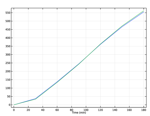
The reference and computed temperatures are compared in Figure 4. The numerical values match the norm values very well.

Figure 4: Reference (blue) and calculated temperature (green).

The exact values, and the absolute and relative errors for each time are listed in Table 2.

Table 2: Results.
Time (min)	Reference temperature(°C)	Calculated temperature(°C)	Absolute error	Relative error
30	36.9	33.4	3.5	9.4
60	137.4	133.9	3.5	2.5
90	244.6	242.9	1.7	0.7
120	361.1	363.0	1.9	0.5
150	466.2	471.1	4.9	1.1
180	554.8	562.0	7.2	1.3

To fulfill the norm, the maximum deviation from the reference values must not exceed 5 K for t ≤ 60 min and 3% for t > 60 min.

Reference

1. DIN EN 1991-1-2/NA, National Annex - Nationally determined parameters - Eurocode 1: Actions on structures - Part 1-2: General actions - Actions on structures exposed to fire

Heat_Transfer_Module/Verification_Examples/fire_effects_heating

Modeling Instructions

From the menu, choose .

New

In the window, click

Model Wizard

In the window, click

In the tree, select .

Click .

Click

In the tree, select .

Click

Geometry 1

Start with creating an interpolation function for the norm values. It will be used later for comparison with the numerical results.

Global Definitions

Reference temperature

In the toolbar, click

and choose .

In the window for , locate the section.

From the list, choose .

Click .

Browse to the model’s Application Libraries folder and double-click the file fire_effects_heating_Tref.txt.

Click .

In the text field, type Reference temperature.

Locate the section. In the text field, type Tref.

Locate the section. In the text field, type min.

In the text field, type degC.

Create another interpolation function for the thermal conductivity.

Thermal conductivity

In the toolbar, click

and choose .

In the window for , type Thermal conductivity in the text field.

Locate the section. In the text field, type k_lin.

In the table, enter the following settings:


t	f(t)
0	1.5
200	0.7
1000	0.5

Locate the section. In the text field, type degC.

In the text field, type W/(m*K).

Click

Geometry 1

Square 1 (sq1)

In the toolbar, click

In the window for , locate the section.

In the text field, type 0.2.

Point 1 (pt1)

In the toolbar, click

In the window for , locate the section.

In the text field, type 0.1.

In the text field, type .1.

Materials

Material 1 (mat1)

In the window, under right-click and choose .

In the window for , locate the section.

In the table, enter the following settings:


Property	Variable	Value	Unit	Property group
Thermal conductivity	k_iso ; kii = k_iso, kij = 0	k_lin(T)	W/(m·K)	Basic
Density	rho	2400	kg/m³	Basic
Heat capacity at constant pressure	Cp	1000	J/(kg·K)	Basic