You are viewing the documentation for an older COMSOL version. The latest version is available here.
PDF

Composite Thermal Barrier
Introduction
This example shows how to set up multiple sandwiched thin layers with different thermal conductivities in two different ways.
First, the composite is modeled as a 3D object. In the second approach, the Thin Layer boundary condition is used to avoid resolving the thin domains, and two modeling options of this feature are compared.
The technique is useful when modeling heat transfer through thermal barriers like multilayer coatings.
See Lumped Composite Thermal Barrier for a comparison of the 3D approach with a 0D approach using the Lumped Thermal System interface.
Model Definition
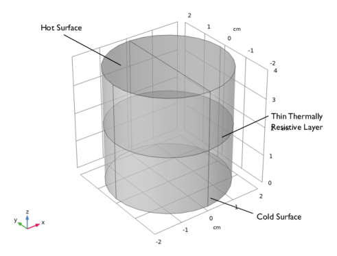
This tutorial uses a simple geometry as shown in Figure 1. The cylinder has a radius of 2 cm and a height of 4 cm.
Figure 1: Geometry.
The composite consists of two layers with different thermal conductivities. The first approach resolves each layer as a 3D domain. The height of the layers is about three orders of magnitude smaller than the bulk height. This often requires to build a mesh manually to accurately resolve the thin structure.
COMSOL Multiphysics provides a special boundary condition which is available from the Heat Transfer Module, namely the Thin Layer feature.
The second approach first uses this feature with resistive property (Thermally thick approximation option). This simplifies the geometry and thus the mesh by representing the thermal barrier as a boundary. In complex geometries, this boundary condition can reduce the amount of memory and time required for the simulation significantly.
The underlying equation assumes the heat flux through the layer proportional to the temperature difference between upper and lower bulk. It is based on the assumption that the bulk on each side is well stirred so that all resistance against heat transfer is within a thin layer near the wall. Due to the additivity of resistance the flux over the composite can be lumped to
where the overall thermal conductivity ktot can be calculated as
Then, the second approach uses the General option of the Thin Layer feature. In this case, an extra-dimension is defined on the boundary to resolve the heat flux both in tangential and normal direction in the layers.
Material Properties
The cylinder is made of steel. The composite consists of two layers of different ceramics.
Boundary Conditions
The temperature at the bottom is fixed to 20°C whereas one half of the top boundary is held at 1220°C (1493 K). All other outer boundaries are perfectly insulated.
Results and Discussion
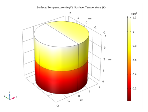
Figure 2 shows the temperature distribution in the cylinder. The composite acts as a thermal barrier resulting in a jump of the temperature over the layer.
Figure 2: Temperature distribution.
Of interest is if the thin layer boundary condition produces reliable results compared to resolving the thin layers in 3D. This can be done with a comparative line graph as in Figure 3. It shows that the 2D approach, with or without a 1D extra dimension, produces accurate results for the bulk temperatures.
Figure 3: Temperature profile for 3D, 2D, and 2D with extra dimension approaches.
Another important question for simulating is the influence on the mesh size and on the required RAM.
With the default tetrahedral mesh the number of mesh elements is about 130,000 elements and the meshing algorithm gives some warnings.
With the swept mesh feature you can significantly reduce the number of elements to about 2,800 elements which is only 2%. In complex geometries the swept mesh algorithm is often not applicable. Using the thin layer boundary condition, the number of mesh elements reduces from 2,800 to 2,000 which is about 30% less, even in this simple geometry. You can see the number of mesh elements used in the Messages window below the Graphics window.
Notes About the COMSOL Implementation
To compare the results directly, both approaches are handled within one mph-file.
Application Library path: Heat_Transfer_Module/Tutorials,_Thin_Structure/composite_thermal_barrier
Modeling Instructions
From the File menu, choose New.
New
In the New window, click  Model Wizard.
Model Wizard
1
In the Model Wizard window, click  3D.
2
In the Select Physics tree, select Heat Transfer>Heat Transfer in Solids (ht).
3
Click Add.
4
Click  Study.
5
In the Select Study tree, select General Studies>Stationary.
6
Global Definitions
Parameters 1
1
In the Model Builder window, under Global Definitions click Parameters 1.
2
In the Settings window for Parameters, locate the Parameters section.
3
Geometry 1
1
In the Model Builder window, under Component 1 (comp1) click Geometry 1.
2
In the Settings window for Geometry, locate the Units section.
3
From the Length unit list, choose cm.
Cylinder 1 (cyl1)
1
In the Geometry toolbar, click  Cylinder.
2
In the Settings window for Cylinder, locate the Size and Shape section.
3
In the Radius text field, type 2.
4
In the Height text field, type 4.
5
In the Geometry toolbar, click  Build All.
Now, create thin cylinders to define the ceramic layers between the two steel domains.
Cylinder 2 (cyl2)
1
In the Geometry toolbar, click  Cylinder.
2
In the Settings window for Cylinder, locate the Size and Shape section.
3
In the Radius text field, type 2.
4
In the Height text field, type d_ceram1.
5
Locate the Position section. In the z text field, type 2-(d_ceram1+d_ceram2)/2.
6
In the Geometry toolbar, click  Build All.
Cylinder 3 (cyl3)
1
In the Geometry toolbar, click  Cylinder.
2
In the Settings window for Cylinder, locate the Size and Shape section.
3
In the Radius text field, type 2.
4
In the Height text field, type d_ceram2.
5
Locate the Position section. In the z text field, type 2-(d_ceram1+d_ceram2)/2+d_ceram1.
6
In the Geometry toolbar, click  Build All.
Polygon 1 (pol1)
1
In the Geometry toolbar, click  More Primitives and choose Polygon.
2
In the Settings window for Polygon, locate the Coordinates section.
3
4
In the Geometry toolbar, click  Build All.
Definitions
Create operators and variables to evaluate the average temperature in the thermal barrier and in each of its layers.
Integration : Barrier
1
In the Model Builder window, expand the Component 1 (comp1)>Definitions node.
2
Right-click Definitions and choose Nonlocal Couplings>Integration.
3
In the Settings window for Integration, locate the Source Selection section.
4
Click  Paste Selection.
5
In the Paste Selection dialog box, type 2 3 in the Selection text field.
6
7
In the Settings window for Integration, type intopBarrier in the Operator name text field.
8
In the Label text field, type Integration : Barrier.
Integration : Layer 1
1
Right-click Integration : Barrier and choose Duplicate.
2
In the Settings window for Integration, locate the Source Selection section.
3
4
Click  Remove from Selection.
5
6
In the Label text field, type Integration : Layer 1.
7
In the Operator name text field, type intopLayer1.
Integration : Layer 2
1
In the Model Builder window, under Component 1 (comp1)>Definitions right-click Integration : Barrier (intopBarrier) and choose Duplicate.
2
In the Settings window for Integration, locate the Source Selection section.
3
4
Click  Remove from Selection.
5
6
In the Label text field, type Integration : Layer 2.
7
In the Operator name text field, type intopLayer2.
Variables: temperature in thermal barrier
1
In the Model Builder window, right-click Definitions and choose Variables.
2
In the Settings window for Variables, locate the Variables section.
3
4
In the Label text field, type Variables: temperature in thermal barrier.
Materials
Material Link 1 (matlnk1)
1
In the Model Builder window, under Component 1 (comp1) right-click Materials and choose More Materials>Material Link.
2
In the Settings window for Material Link, locate the Link Settings section.
3
Click  Add Material from Library.
Add Material to Material Link 1 (matlnk1)
1
Go to the Add Material to Material Link 1 (matlnk1) window.
2
In the tree, select Built-in>Steel AISI 4340.
3
Click  Add to Material Link 1 (matlnk1).
Materials
Material Link 2 (matlnk2)
1
Right-click Materials and choose More Materials>Material Link.
2
In the Settings window for Material Link, locate the Geometric Entity Selection section.
3
Click  Paste Selection.
4
In the Paste Selection dialog box, type 2 in the Selection text field.
5
6
In the Settings window for Material Link, locate the Link Settings section.
7
Click  Blank Material.
8
In the Model Builder window, click Material Link 2 (matlnk2).
9
Click  Go to Material.
Global Definitions
Ceramic 1
1
In the Model Builder window, under Global Definitions>Materials click Material 2 (mat2).
2
In the Settings window for Material, type Ceramic 1 in the Label text field.
3
Locate the Material Contents section. In the table, enter the following settings:
Materials
Material Link 3 (matlnk3)
1
In the Model Builder window, under Component 1 (comp1) right-click Materials and choose More Materials>Material Link.
2
In the Settings window for Material Link, locate the Geometric Entity Selection section.
3
Click  Paste Selection.
4
In the Paste Selection dialog box, type 3 in the Selection text field.
5
6
In the Settings window for Material Link, locate the Link Settings section.
7
Click  Blank Material.
8
In the Model Builder window, click Material Link 3 (matlnk3).
9
Click  Go to Material.
Global Definitions
Ceramic 2
1
In the Model Builder window, under Global Definitions>Materials click Material 3 (mat3).
2
In the Settings window for Material, type Ceramic 2 in the Label text field.
3
Locate the Material Contents section. In the table, enter the following settings:
Heat Transfer in Solids (ht)
Temperature 1
1
In the Model Builder window, under Component 1 (comp1) right-click Heat Transfer in Solids (ht) and choose Temperature.
2
Temperature 2
1
In the Physics toolbar, click  Boundaries and choose Temperature.
2
3
In the Settings window for Temperature, locate the Temperature section.
4
In the T0 text field, type T_hot.
Mesh 1
First, mesh the top surface with a free triangular mesh and extrude it in layers through the cylindrical geometry. With a Distribution node, specify how many mesh layers are to be created within the domain. Resolve the composite layers with two elements in thickness.
Free Triangular 1
1
In the Mesh toolbar, click  Boundary and choose Free Triangular.
2
3
In the Settings window for Free Triangular, click  Build Selected.
Swept 1
In the Mesh toolbar, click  Swept.
Distribution 1
1
Right-click Swept 1 and choose Distribution.
2
3
In the Settings window for Distribution, locate the Distribution section.
4
In the Number of elements text field, type 2.
5
Click  Build All.
Study 1
In the Home toolbar, click  Compute.
Results
Temperature (ht)
The following plots are produced by default: temperature profile on the surface as in Figure 2, and isothermal contours.
Surface
1
In the Model Builder window, expand the Temperature (ht) node, then click Surface.
2
In the Settings window for Surface, locate the Expression section.
3
From the Unit list, choose degC.
4
In the Temperature (ht) toolbar, click  Plot.
Next, create a temperature profile along the height of the cylinder. You will later compare the graph with the results of the 2D approach.
Temperature Profile
1
In the Home toolbar, click  Add Plot Group and choose 1D Plot Group.
2
In the Settings window for 1D Plot Group, type Temperature Profile in the Label text field.
3
Locate the Plot Settings section. Select the x-axis label check box.
4
5
Click to expand the Title section. From the Title type list, choose Manual.
6
In the Title text area, type Temperature Profile.
7
Locate the Legend section. From the Position list, choose Upper left.
Line Graph 1
1
In the Temperature Profile toolbar, click  Line Graph.
2
3
In the Settings window for Line Graph, locate the y-Axis Data section.
4
From the Unit list, choose degC.
5
Locate the x-Axis Data section. From the Parameter list, choose Expression.
6
In the Expression text field, type z.
7
Click to expand the Coloring and Style section. In the Width text field, type 2.
8
Click to expand the Legends section. Select the Show legends check box.
9
From the Legends list, choose Manual.
10
11
In the Temperature Profile toolbar, click  Plot.
Group the plots corresponding to the 3D approach under a single node.
3D Approach
1
In the Model Builder window, right-click Results and choose Node Group.
2
In the Settings window for Group, type 3D Approach in the Label text field.
Isothermal Contours (ht)
Now let all the plots being regenerated after solving.
1
In the Model Builder window, click Results.
2
In the Settings window for Results, locate the Update of Results section.
3
Select the Recompute all plot data after solving check box.
Create now the second model which uses the Thin Layer feature and compare the results to the first approach.
Add Component
In the Model Builder window, right-click the root node and choose Add Component>3D.
Add Physics
1
In the Home toolbar, click  Add Physics to open the Add Physics window.
2
Go to the Add Physics window.
3
In the tree, select Heat Transfer>Heat Transfer in Solids (ht).
4
Find the Physics interfaces in study subsection. In the table, clear the Solve check box for Study 1.
5
Click Add to Component 2 in the window toolbar.
6
In the Home toolbar, click  Add Physics to close the Add Physics window.
Add Study
1
In the Home toolbar, click  Add Study to open the Add Study window.
2
Go to the Add Study window.
3
Find the Studies subsection. In the Select Study tree, select General Studies>Stationary.
4
Find the Physics interfaces in study subsection. In the table, clear the Solve check box for Heat Transfer in Solids (ht).
5
Click Add Study in the window toolbar.
6
In the Model Builder window, click the root node.
7
In the Home toolbar, click  Add Study to close the Add Study window.
Geometry 2
1
In the Settings window for Geometry, locate the Units section.
2
From the Length unit list, choose cm.
Cylinder 1 (cyl1)
1
Right-click Component 2 (comp2)>Geometry 2 and choose Cylinder.
2
In the Settings window for Cylinder, locate the Size and Shape section.
3
In the Radius text field, type 2.
4
In the Height text field, type 4.
5
Click to expand the Layers section. In the table, enter the following settings:
6
Clear the Layers on side check box.
7
Select the Layers on bottom check box.
8
In the Geometry toolbar, click  Build All.
Polygon 1 (pol1)
1
In the Geometry toolbar, click  More Primitives and choose Polygon.
2
In the Settings window for Polygon, locate the Coordinates section.
3
4
In the Geometry toolbar, click  Build All.
Definitions (comp2)
In order to make the comparison with Component 1, create an Integration operator and variables to evaluate the average temperature in the thermal barrier and in each of its layers.
Integration : Boundary
1
In the Model Builder window, expand the Component 2 (comp2)>Definitions node.
2
Right-click Component 2 (comp2)>Definitions and choose Nonlocal Couplings>Integration.
3
In the Settings window for Integration, type Integration : Boundary in the Label text field.
4
In the Operator name text field, type intopBnd.
5
Locate the Source Selection section. From the Geometric entity level list, choose Boundary.
6
Click  Paste Selection.
7
In the Paste Selection dialog box, type 6 in the Selection text field.
8
Variables: temperature in thermal barrier
1
Right-click Definitions and choose Variables.
2
In the Settings window for Variables, locate the Variables section.
3
4
In the Label text field, type Variables: temperature in thermal barrier.
Materials
Material Link 4 (matlnk4)
In the Model Builder window, under Component 2 (comp2) right-click Materials and choose More Materials>Material Link.
Global Definitions
Layered Material 1 (lmat1)
1
In the Model Builder window, under Global Definitions right-click Materials and choose Layered Material.
2
In the Settings window for Layered Material, locate the Layer Definition section.
3
4
5
Materials
Layered Material Link 1 (llmat1)
1
In the Model Builder window, under Component 2 (comp2) right-click Materials and choose Layers>Layered Material Link.
2
Heat Transfer in Solids 2 (ht2)
Add two Thin Layer nodes on the same boundary. They will be activated each in two separated studies, to compare the Thermally thick approximation and General options.
1
In the Model Builder window, under Component 2 (comp2) click Heat Transfer in Solids 2 (ht2).
Thin Layer 1
1
In the Physics toolbar, click  Boundaries and choose Thin Layer.
2
Thin Layer 2
1
In the Physics toolbar, click  Boundaries and choose Thin Layer.
2
3
In the Settings window for Thin Layer, locate the Layer Model section.
4
From the Layer type list, choose General.
Temperature 1
1
In the Physics toolbar, click  Boundaries and choose Temperature.
2
Temperature 2
1
In the Physics toolbar, click  Boundaries and choose Temperature.
2
3
In the Settings window for Temperature, locate the Temperature section.
4
In the T0 text field, type T_hot.
Study 2
Step 1: Stationary
1
In the Model Builder window, under Study 2 click Step 1: Stationary.
2
In the Settings window for Stationary, locate the Physics and Variables Selection section.
3
Select the Modify model configuration for study step check box.
Disable Thin Layer 2 in this study. First, Thin Layer 1 is used to show the results with the Thermally thick approximation option. Later, another study will use Thin Layer 2 with the General option.
4
In the Physics and variables selection tree, select Component 2 (comp2)>Heat Transfer in Solids 2 (ht2)>Thin Layer 2.
5
Click  Disable.
Mesh 2
In the Model Builder window, under Component 2 (comp2) click Mesh 2.
Free Triangular 1
1
In the Mesh toolbar, click  Boundary and choose Free Triangular.
2
3
In the Settings window for Free Triangular, click  Build Selected.
Swept 1
1
In the Mesh toolbar, click  Swept.
2
In the Model Builder window, right-click Mesh 2 and choose Build All.
Study 2
In the Home toolbar, click  Compute.
Results
Surface 1
1
In the Model Builder window, expand the Temperature (ht2) node, then click Surface 1.
2
In the Settings window for Surface, locate the Expression section.
3
From the Unit list, choose degC.
Temperature Profile
In the Model Builder window, click Temperature Profile.
Line Graph 2
1
Right-click Temperature Profile and choose Line Graph.
2
In the Settings window for Line Graph, locate the Data section.
3
From the Dataset list, choose Study 2/Solution 2 (3) (sol2).
4
5
Click Replace Expression in the upper-right corner of the y-Axis Data section. From the menu, choose Component 2 (comp2)>Heat Transfer in Solids 2>Temperature>T2 - Temperature - K.
6
Locate the y-Axis Data section. From the Unit list, choose degC.
7
Locate the x-Axis Data section. From the Parameter list, choose Expression.
8
In the Expression text field, type z.
9
Locate the Coloring and Style section. Find the Line style subsection. From the Line list, choose None.
10
From the Color list, choose Magenta.
11
Find the Line markers subsection. From the Marker list, choose Cycle.
12
In the Number text field, type 15.
13
Locate the Legends section. Select the Show legends check box.
14
From the Legends list, choose Manual.
15
16
In the Temperature Profile toolbar, click  Plot.
Surface 2
1
In the Model Builder window, click Surface 2.
2
In the Settings window for Surface, locate the Expression section.
3
From the Unit list, choose degC.
Group the plots corresponding to the 2D approach under a single node.
2D Approach
1
In the Model Builder window, right-click Results and choose Node Group.
2
In the Settings window for Group, type 2D Approach in the Label text field.
Isothermal Contours (ht2)
Next, add a study to solve Component 2 with Thin Layer 2 instead of Thin Layer 1. The Thin Layer 2 feature would use the General option which creates a 1D extra dimension formed by two intervals to represent the two ceramic layers.
Add Study
1
In the Home toolbar, click  Add Study to open the Add Study window.
2
Go to the Add Study window.
3
Find the Studies subsection. In the Select Study tree, select General Studies>Stationary.
4
Find the Physics interfaces in study subsection. In the table, clear the Solve check box for Heat Transfer in Solids (ht).
5
Click Add Study in the window toolbar.
6
In the Home toolbar, click  Add Study to close the Add Study window.
Study 3
Step 1: Stationary
1
In the Settings window for Stationary, locate the Physics and Variables Selection section.
2
Select the Modify model configuration for study step check box.
3
In the Physics and variables selection tree, select Component 2 (comp2)>Heat Transfer in Solids 2 (ht2)>Thin Layer 1.
4
Click  Disable.
5
In the Home toolbar, click  Compute.
Results
Surface 1
1
In the Model Builder window, expand the Temperature (ht2) 1 node, then click Surface 1.
2
In the Settings window for Surface, locate the Expression section.
3
From the Unit list, choose degC.
Surface 2
1
In the Model Builder window, click Surface 2.
2
In the Settings window for Surface, locate the Expression section.
3
From the Unit list, choose degC.
Temperature Profile
In the Model Builder window, click Temperature Profile.
Line Graph 3
1
In the Temperature Profile toolbar, click  Line Graph.
2
In the Settings window for Line Graph, locate the Data section.
3
From the Dataset list, choose Study 3/Solution 3 (5) (sol3).
4
5
Locate the y-Axis Data section. In the Expression text field, type T2.
6
From the Unit list, choose degC.
7
Locate the x-Axis Data section. From the Parameter list, choose Expression.
8
In the Expression text field, type z.
9
Locate the Coloring and Style section. Find the Line style subsection. From the Line list, choose None.
10
From the Color list, choose Black.
11
In the Width text field, type 2.
12
Find the Line markers subsection. From the Marker list, choose Triangle.
13
In the Number text field, type 20.
14
Locate the Legends section. Select the Show legends check box.
15
From the Legends list, choose Manual.
16
17
In the Temperature Profile toolbar, click  Plot.
The plot should look like that in Figure 3.
Group the plots corresponding to the 2D with extra dimension approach under a single node.
2D With Extra Dimension Approach
1
In the Model Builder window, right-click Results and choose Node Group.
2
In the Settings window for Group, type 2D With Extra Dimension Approach in the Label text field.
Isothermal Contours (ht2) 1
Also, place the plot comparing the different approaches under a specific node.
Comparison of the Different Approaches
1
Right-click Results and choose Node Group.
2
In the Settings window for Group, type Comparison of the Different Approaches in the Label text field.
Temperature Profile
Next, create plots to compare more in details the results obtained with Study 1 and Study 3 for the temperature in the ceramic layers. In addition, evaluate the average of the thermal barrier temperature obtained with these two studies.
First, create a plot for the temperature solution at the surface of the thermal barrier.
Temperature (Layers Surface)
1
In the Home toolbar, click  Add Plot Group and choose 3D Plot Group.
2
In the Settings window for 3D Plot Group, type Temperature (Layers Surface) in the Label text field.
3
Locate the Data section. From the Dataset list, choose Layered Material 2.
Surface 1
1
Right-click Temperature (Layers Surface) and choose Surface.
2
In the Settings window for Surface, locate the Expression section.
3
From the Unit list, choose degC.
4
Locate the Coloring and Style section. From the Color table list, choose ThermalLight.
5
In the Temperature (Layers Surface) toolbar, click  Plot.
For a better rendering, change the scaling factor for the thickness of the layers in the Layered Material 2 dataset.
Layered Material 2
1
In the Model Builder window, expand the Results>Datasets node, then click Layered Material 2.
2
In the Settings window for Layered Material, locate the Layers section.
3
In the Scale text field, type 20.
4
Temperature (Layers Surface)
1
In the Model Builder window, click Temperature (Layers Surface).
2
In the Settings window for 3D Plot Group, locate the Plot Settings section.
3
From the View list, choose New view.
2D With Extra Dimension Approach
Next, create a plot for the temperature on slices of the thermal barrier.
Temperature (Slices)
1
In the Home toolbar, click  Add Plot Group and choose 3D Plot Group.
2
In the Settings window for 3D Plot Group, type Temperature (Slices) in the Label text field.
3
Locate the Data section. From the Dataset list, choose Study 3/Solution 3 (5) (sol3).
4
Locate the Plot Settings section. Clear the Plot dataset edges check box.
5
From the View list, choose New view.
Layered Material Slice 1
1
Right-click Temperature (Slices) and choose Layered Material Slice.
2
In the Settings window for Layered Material Slice, locate the Expression section.
3
From the Unit list, choose degC.
4
Locate the Through-Thickness Location section. From the Location definition list, choose Interfaces.
5
Locate the Layout section. From the Displacement list, choose Linear.
6
From the Orientation list, choose x.
7
In the Relative x-separation text field, type 0.25.
8
Select the Show descriptions check box.
9
In the Relative separation text field, type 1.
10
Locate the Coloring and Style section. From the Color table list, choose ThermalLight.
11
In the Temperature (Slices) toolbar, click  Plot.
12
Click the  Zoom Extents button in the Graphics toolbar.
Next, plot the temperature through the thickness of the thermal barrier.
Temperature (Through Thickness)
1
In the Home toolbar, click  Add Plot Group and choose 1D Plot Group.
2
In the Settings window for 1D Plot Group, type Temperature (Through Thickness) in the Label text field.
Line Graph 1
1
Right-click Temperature (Through Thickness) and choose Line Graph.
2
3
In the Settings window for Line Graph, locate the y-Axis Data section.
4
In the Expression text field, type z-(2[cm]-(d_ceram1+d_ceram2)/2).
5
From the Unit list, choose m.
6
Locate the x-Axis Data section. From the Parameter list, choose Expression.
7
From the Unit list, choose degC.
Temperature (Through Thickness)
In the Model Builder window, click Temperature (Through Thickness).
Through Thickness 1
1
In the Temperature (Through Thickness) toolbar, click  More Plots and choose Through Thickness.
2
In the Settings window for Through Thickness, locate the Data section.
3
From the Dataset list, choose Study 3/Solution 3 (5) (sol3).
4
5
Locate the x-Axis Data section. In the Expression text field, type T2.
6
From the Unit list, choose degC.
7
Click to expand the Coloring and Style section. Find the Line style subsection. From the Line list, choose None.
8
Find the Line markers subsection. From the Marker list, choose Cycle.
9
Locate the y-Axis Data section. Find the Interface positions subsection. From the Show interface positions list, choose All interfaces.
10
In the Temperature (Through Thickness) toolbar, click  Plot.
Temperature (Through Thickness)
Finally, evaluate the average temperature in the thermal barrier and in each of its layers by making a Global Evaluation of the variables defined previously in each component.
Global Evaluation 1
1
In the Results toolbar, click  Global Evaluation.
2
In the Settings window for Global Evaluation, click Replace Expression in the upper-right corner of the Expressions section. From the menu, choose Component 1 (comp1)>Definitions>Variables>T_ave_barrier - Average of temperature in thermal barrier - K.
3
Click Add Expression in the upper-right corner of the Expressions section. From the menu, choose Component 1 (comp1)>Definitions>Variables>T_ave_layer1 - Average of temperature in layer 1 - K.
4
Click Add Expression in the upper-right corner of the Expressions section. From the menu, choose Component 1 (comp1)>Definitions>Variables>T_ave_layer2 - Average of temperature in layer 2 - K.
5
Locate the Expressions section. In the table, enter the following settings:
6
Click  Evaluate.
Global Evaluation 2
1
In the Results toolbar, click  Global Evaluation.
2
In the Settings window for Global Evaluation, locate the Data section.
3
From the Dataset list, choose Study 3/Solution 3 (5) (sol3).
4
Click Replace Expression in the upper-right corner of the Expressions section. From the menu, choose Component 2 (comp2)>Definitions>Variables>T_ave_barrier - Average of temperature in thermal barrier - K.
5
Click Add Expression in the upper-right corner of the Expressions section. From the menu, choose Component 2 (comp2)>Definitions>Variables>T_ave_layer1 - Average of temperature in layer 1 - K.
6
Click Add Expression in the upper-right corner of the Expressions section. From the menu, choose Component 2 (comp2)>Definitions>Variables>T_ave_layer2 - Average of temperature in layer 2 - K.
7
Locate the Expressions section. In the table, enter the following settings:
8
Click  Evaluate.
The average temperature is close to 530°C in the thermal barrier, with some noticeable difference between the two layers.