PDF

Fuel Cell with Serpentine Flow Field
Introduction
The design of the fuel cell flow pattern governs the fuel utilization, the current distribution, and the pressure drop in the cell. A common design approach is to use serpentine channels in order to evenly distribute the reacting fluid over the electrode area. The serpentine design has the advantage of creating a set of parallel channels of equal length and similar flow resistances for a small inlet manifold. However, the design may induce unnecessarily high pressure drops. Also, for low temperature fuel cells, clogging due to water condensation may occur in the serpentine bends.
For the serpentine channel design to work properly, the channel-to-channel cross-flow, due to in-plane convection in the underlaying porous material layer, should be moderate, since large cross-flow may lead to stagnant zones and uneven flow between the channels.
This example describes the cathode airflow and mass transport in three serpentine channels and the underlying gas diffusion layer (GDL) of a polymer electrolyte fuel cell.
The same model parameters are used as in the Mass Transport Analysis of a High Temperature PEM Fuel Cell example.
Model Definition
The model geometry is show in Figure 1. The model consists of three channel domains on the cathode (oxygen) side, and the underlying cathode GDL, membrane and anode GDL domains. The channel inlets are on the left and the outlets on the right. The bottom anode GDL boundary faces the anode flow channels which are not included in the model geometry.
Figure 1: Model geometry.
The current distribution and the mass transport are modeled using a Hydrogen Fuel Cell interface. This physics interface solves for the electrolyte and electrode phase potentials, as well as the molar fraction of oxygen, nitrogen and water on the cathode side. The momentum transfer is solved for using a Free and Porous Media flow interface. This physics interface solves for the fluid velocity and pressures. The fuel cell and the flow interfaces are coupled together using a Reacting Flow, O2 Gas Phase which couples the velocity field, pressure gradient as well as the composition dependent density and viscosity between the two interfaces.
The porous cathode reaction reduces oxygen according to
This reaction is modeled as a Thin Gas Diffusion Electrode in combination with a Thin Gas Diffusion Electrode Reaction subnode. The local current density, iloc (SI unit: A/m2) depends on the oxygen concentration and the local overpotential according to the following kinetic expression:
O2 Inlet and O2 Outlet are used on the inlet and outlet boundaries, respectively. No slip wall conditions are used for the channel walls, whereas slip conditions are used for the GDL walls.
On the anode side, the gas stream is assumed to be unaffected by the electrode reactions in the cell, consisting of 100% hydrogen within the whole of the anode GDL and gas diffusion electrode.
The anode current collector boundary is grounded, whereas a cell potential is prescribed to the cathode current collector boundaries.
The mesh is shown in Figure 2. The bottom channel, and the GDL area between the serpentine bend of the bottom channel have a finer mesh in order to resolve the channel-to-channel cross-flow.
Figure 2: Mesh.
The problem is solved in three consecutive study steps: The first steps solves for the potentials only, the second step solves for the velocity and pressure only, and the final step solves for the full problem, solving for the cell potentials 1, 0.7 and 0.5 V.
Results and Discussion
Figure 3 shows the velocity magnitude in the cell. There is a small channel-to-channel leakage in the GDL
Figure 3: Velocity magnitude. Left: Slice plot in the middle of the channels. Right: Slice plot in the middle of the GDL.
Figure 4 shows the oxygen molar fraction in the gas stream at a cell voltage at 0.7 and 0.5 V. The oxygen level decreases towards the outlet in both cases, with generally lower levels at 0.5 V.
Figure 4: Oxygen mole fraction at 0.7 V (left) and 0.5 V (right)
Figure 5 shows the corresponding electrolyte current density in the z-direction at the cathode. The currents densities are generally higher at 0.5 V, and less uniform. The current densities decrease towards the outlet which can be explained by the lower oxygen concentration levels shown in Figure 4. A minor effect of the GDL channel-to-channel leakage flow can be observed.
Figure 5: Electrolyte current density at the cathode in the z-direction at 0.7 V (left) and 0.5 V (right)
Application Library path: Fuel_Cell_and_Electrolyzer_Module/Fuel_Cells/serpentine_flow_field
Modeling Instructions
From the File menu, choose New.
New
In the New window, click  Model Wizard.
Model Wizard
1
In the Model Wizard window, click  3D.
2
In the Select Physics tree, select Electrochemistry>Hydrogen Fuel Cells>Proton Exchange (fc).
3
Click Add.
4
In the Select Physics tree, select Fluid Flow>Porous Media and Subsurface Flow>Free and Porous Media Flow (fp).
5
Click Add.
6
Click  Study.
7
In the Select Study tree, select Preset Studies for Selected Physics Interfaces>Hydrogen Fuel Cell>Stationary with Initialization.
8
Geometry 1
The model geometry is available as a parameterized geometry sequence in a separate MPH-file. If you want to build it from scratch, follow the instructions in the section Appendix — Geometry Modeling Instructions. Otherwise load it from file with the following steps.
1
In the Geometry toolbar, click  Insert Sequence.
2
3
In the Geometry toolbar, click  Build All.
4
In the Model Builder window, collapse the Geometry 1 node.
Global Definitions
The insertion of the geometry sequence added some parameters to the model. Load some additional physics parameters a text files.
Geometry Parameters
1
In the Model Builder window, under Global Definitions click Parameters 1.
2
In the Settings window for Parameters, type Geometry Parameters in the Label text field.
Physics Parameters
1
In the Home toolbar, click  Parameters and choose Add>Parameters.
2
In the Settings window for Parameters, type Physics Parameters in the Label text field.
3
Locate the Parameters section. Click  Load from File.
4
Multiphysics
Start setting up the physics. First add a Multiphysics node to couple the two interfaces together.
Reacting Flow, O2 Gas Phase 1 (rfo1)
In the Physics toolbar, click  Multiphysics Couplings and choose Domain>Reacting Flow, O2 Gas Phase.
Hydrogen Fuel Cell (fc)
Next set up the Hydrogen Fuel Cell interface.
In this model, we will not model hydrogen transport on the anode side, assuming a gas consisting of 100% hydrogen.
1
In the Model Builder window, under Component 1 (comp1) click Hydrogen Fuel Cell (fc).
2
In the Settings window for Hydrogen Fuel Cell, locate the H2 Gas Mixture section.
3
Clear the H2O check box.
Membrane 1
Start adding the different domain nodes of the fuel cell model, and assign them to the geometry.
1
In the Physics toolbar, click  Domains and choose Membrane.
2
In the Settings window for Membrane, locate the Domain Selection section.
3
From the Selection list, choose Membrane.
The named selections of the geometry for Membrane etc were created in the geometry sequence.
H2 Gas Diffusion Layer 1
1
In the Physics toolbar, click  Domains and choose H2 Gas Diffusion Layer.
2
In the Settings window for H2 Gas Diffusion Layer, locate the Domain Selection section.
3
From the Selection list, choose H2 GDL.
4
Locate the Electrode Charge Transport section. In the σs text field, type sigma_gdl.
O2 Gas Diffusion Layer 1
1
In the Physics toolbar, click  Domains and choose O2 Gas Diffusion Layer.
2
In the Settings window for O2 Gas Diffusion Layer, locate the Domain Selection section.
3
From the Selection list, choose O2 GDL.
4
Locate the Electrode Charge Transport section. In the σs text field, type sigma_gdl.
5
Locate the Gas Transport section. In the εg text field, type eps_gdl.
Thin H2 Gas Diffusion Electrode 1
1
In the Physics toolbar, click  Boundaries and choose Thin H2 Gas Diffusion Electrode.
2
In the Settings window for Thin H2 Gas Diffusion Electrode, locate the Boundary Selection section.
3
From the Selection list, choose GDE, H2 Side.
4
Locate the Electrode Thickness section. In the dgde text field, type H_electrode.
Thin H2 Gas Diffusion Electrode Reaction 1
1
In the Model Builder window, expand the Thin H2 Gas Diffusion Electrode 1 node, then click Thin H2 Gas Diffusion Electrode Reaction 1.
2
In the Settings window for Thin H2 Gas Diffusion Electrode Reaction, locate the Electrode Kinetics section.
3
In the i0,ref(T) text field, type i0_H2_ref.
4
In the αa text field, type alpha_a_H2.
5
Locate the Active Specific Surface Area section. In the av text field, type Av.
Thin O2 Gas Diffusion Electrode 1
1
In the Physics toolbar, click  Boundaries and choose Thin O2 Gas Diffusion Electrode.
2
In the Settings window for Thin O2 Gas Diffusion Electrode, locate the Boundary Selection section.
3
From the Selection list, choose GDE, O2 Side.
4
Locate the Electrode Thickness section. In the dgde text field, type H_electrode.
Thin O2 Gas Diffusion Electrode Reaction 1
1
In the Model Builder window, expand the Thin O2 Gas Diffusion Electrode 1 node, then click Thin O2 Gas Diffusion Electrode Reaction 1.
2
In the Settings window for Thin O2 Gas Diffusion Electrode Reaction, locate the Electrode Kinetics section.
3
In the i0,ref(T) text field, type i0_O2_ref.
4
In the αa text field, type alpha_a_O2.
5
Locate the Active Specific Surface Area section. In the av text field, type Av.
O2 Flow Channel 1
1
In the Physics toolbar, click  Domains and choose O2 Flow Channel.
2
In the Settings window for O2 Flow Channel, locate the Domain Selection section.
3
From the Selection list, choose O2 Flow Channel.
Continuity 1
In order to be able to use Sweep meshing operations in the through-plane direction of the cell geometry, the geometry node was created as an assembly of the oxygen and hydrogen side, with a dividing plane in the middle of the membrane. A Continuity node is hence needed in order to connect the electrolyte phase equations on each side of the assembly pair boundary.
1
In the Physics toolbar, click  Pairs and choose Continuity.
2
In the Settings window for Continuity, locate the Pair Selection section.
3
Under Pairs, click  Add.
4
In the Add dialog box, select Identity Boundary Pair 1 (ap1) in the Pairs list.
5
Electrolyte Phase 1
Now go back and edit the default phase domain nodes. Also set up the boundary conditions and initial values.
1
In the Model Builder window, click Electrolyte Phase 1.
2
In the Settings window for Electrolyte Phase, locate the Electrolyte Charge Transport section.
3
In the σl text field, type sigma_l.
Electronic Conducting Phase 1
In the Model Builder window, expand the Component 1 (comp1)>Hydrogen Fuel Cell (fc)>Electronic Conducting Phase 1 node, then click Electronic Conducting Phase 1.
Electric Ground 1
1
In the Physics toolbar, click  Attributes and choose Electric Ground.
2
In the Settings window for Electric Ground, locate the Boundary Selection section.
3
From the Selection list, choose H2 Current Collector.
Electronic Conducting Phase 1
In the Model Builder window, click Electronic Conducting Phase 1.
Electric Potential 1
1
In the Physics toolbar, click  Attributes and choose Electric Potential.
2
In the Settings window for Electric Potential, locate the Boundary Selection section.
3
From the Selection list, choose O2 Current Collector.
4
Locate the Electric Potential section. In the φs,bnd text field, type E_cell.
The E_cell parameter will be used by the Auxiliary sweep in the Study in order to solve for a range of potentials.
O2 Gas Phase 1
In the Model Builder window, click O2 Gas Phase 1.
O2 Inlet 1
1
In the Physics toolbar, click  Attributes and choose O2 Inlet.
2
In the Settings window for O2 Inlet, locate the Boundary Selection section.
3
From the Selection list, choose Inlets, O2 side.
4
Locate the Mixture Specification section. In the x0,H2O text field, type x_H2O_in.
5
In the x0,N2 text field, type x_N2_in.
O2 Gas Phase 1
In the Model Builder window, click O2 Gas Phase 1.
O2 Outlet 1
1
In the Physics toolbar, click  Attributes and choose O2 Outlet.
2
In the Settings window for O2 Outlet, locate the Boundary Selection section.
3
From the Selection list, choose Outlets, O2 side.
Initial Values 1
1
In the Model Builder window, click Initial Values 1.
2
In the Settings window for Initial Values, locate the Initial Values section.
3
In the x0,H2O text field, type x_H2O_in.
4
In the x0,N2 text field, type x_N2_in.
The fuel cell settings are now complete.
Free and Porous Media Flow (fp)
Next, set up the Free and Porous Media Flow interface.
1
In the Model Builder window, under Component 1 (comp1) click Free and Porous Media Flow (fp).
2
In the Settings window for Free and Porous Media Flow, locate the Domain Selection section.
3
From the Selection list, choose O2 Flow Domains.
4
Locate the Physical Model section. From the Compressibility list, choose Weakly compressible flow.
The weakly compressible option is suitable when density changes due to pressure gradients are expected to be relatively small.
Fluid and Matrix Properties 1
1
In the Model Builder window, expand the Free and Porous Media Flow (fp) node.
2
Right-click Free and Porous Media Flow (fp) and choose Fluid and Matrix Properties.
3
In the Settings window for Fluid and Matrix Properties, locate the Domain Selection section.
4
From the Selection list, choose O2 GDL.
5
Locate the Porous Matrix Properties section. From the εp list, choose User defined. In the associated text field, type eps_gdl.
6
From the κ list, choose User defined. In the associated text field, type kappa_gdl.
Inlet 1
1
In the Physics toolbar, click  Boundaries and choose Inlet.
2
In the Settings window for Inlet, locate the Boundary Selection section.
3
From the Selection list, choose Inlets, O2 side.
4
Locate the Boundary Condition section. From the list, choose Fully developed flow.
5
Clear the Apply condition on each disjoint selection separately check box.
6
Locate the Fully Developed Flow section. In the Uav text field, type U_in.
Outlet 1
1
In the Physics toolbar, click  Boundaries and choose Outlet.
2
In the Settings window for Outlet, locate the Boundary Selection section.
3
From the Selection list, choose Outlets, O2 side.
Wall 2
1
In the Physics toolbar, click  Boundaries and choose Wall.
2
In the Settings window for Wall, locate the Boundary Selection section.
3
From the Selection list, choose Slip Walls.
4
Locate the Boundary Condition section. From the Wall condition list, choose Slip.
Setting the external walls of the porous domain to slip conditions improves the convergence for this model.
Global Definitions
Finalize the physics settings by setting the temperature on the Default Model Inputs node. This setting will be used by all physics.
Default Model Inputs
1
In the Model Builder window, under Global Definitions click Default Model Inputs.
2
In the Settings window for Default Model Inputs, locate the Browse Model Inputs section.
3
In the tree, select General>Temperature (K) - minput.T.
4
Find the Expression for remaining selection subsection. In the Temperature text field, type T.
Mesh 1
A model geometry of this complexity benefits from manual meshing. The manually created mesh will improve convergence and reduce computational time.
1
In the Model Builder window, under Component 1 (comp1) click Mesh 1.
2
In the Settings window for Mesh, locate the Physics-Controlled Mesh section.
3
From the Element size list, choose Finer.
Mapped 1
The straight parts of the channels are suitable for sweeping. Start by creating mapped meshes on the start and end faces.
1
In the Mesh toolbar, click  Boundary and choose Mapped.
2
In the Settings window for Mapped, locate the Boundary Selection section.
3
From the Selection list, choose Channel Mesh Sweep Faces.
Distribution 1
1
Right-click Mapped 1 and choose Distribution.
2
In the Settings window for Distribution, locate the Edge Selection section.
3
From the Selection list, choose All edges.
4
Locate the Distribution section. In the Number of elements text field, type 4.
Swept 1
1
In the Mesh toolbar, click  Swept.
2
In the Settings window for Swept, locate the Domain Selection section.
3
From the Geometric entity level list, choose Domain.
4
From the Selection list, choose Channel Sweep Mesh Domains.
Size 1
1
Right-click Swept 1 and choose Size.
2
In the Settings window for Size, locate the Element Size section.
3
Click the Custom button.
4
Locate the Element Size Parameters section. Select the Maximum element size check box.
5
6
Click  Build Selected.
Free Tetrahedral 1
Use a free tetrahedral mesh for the curved parts of the flow channels.
1
In the Mesh toolbar, click  Free Tetrahedral.
2
In the Settings window for Free Tetrahedral, locate the Domain Selection section.
3
From the Geometric entity level list, choose Domain.
4
From the Selection list, choose Channel Tet Mesh Domains.
Size 1
1
Right-click Free Tetrahedral 1 and choose Size.
2
In the Settings window for Size, locate the Element Size section.
3
Click the Custom button.
4
Locate the Element Size Parameters section. Select the Maximum element size check box.
5
6
Click  Build Selected.
Boundary Layers 1
Now add boundary layers inside the channels. The boundary layers will resolve the gradients in velocity close to the channel walls.
1
In the Mesh toolbar, click  Boundary Layers.
2
In the Settings window for Boundary Layers, locate the Geometric Entity Selection section.
3
From the Geometric entity level list, choose Domain.
4
From the Selection list, choose Channels.
Boundary Layer Properties
1
In the Model Builder window, click Boundary Layer Properties.
2
In the Settings window for Boundary Layer Properties, locate the Boundary Selection section.
3
From the Selection list, choose Boundary Layer Walls.
4
Locate the Boundary Layer Properties section. In the Number of boundary layers text field, type 2.
5
In the Boundary layer stretching factor text field, type 1.5.
6
From the Thickness of first layer list, choose Manual.
7
In the Thickness text field, type W_ch/10.
8
Click  Build Selected.
At this point you might want to zoom in the graphics window and inspect the inlet and outlets of the channels to see the created boundary layers.
Now continue to build a surface mesh for the upper GDL boundary. The mesh will then be swept in the through-plane direction for the remaining domains of the oxygen side of the assembly geometry.
9
Click the  Go to XY View button in the Graphics toolbar.
Mapped 2
1
In the Mesh toolbar, click  Boundary and choose Mapped.
2
In the Settings window for Mapped, locate the Boundary Selection section.
3
From the Selection list, choose O2 Current Collector Mapped Mesh Boundaries.
4
Click  Build Selected.
Free Triangular 1
1
In the Mesh toolbar, click  Boundary and choose Free Triangular.
2
In the Settings window for Free Triangular, locate the Boundary Selection section.
3
From the Selection list, choose O2 Current Collector Triangular Mesh Boundaries.
4
Click  Build Selected.
Boundary Layers 2
Add a boundary layer also to the surface mesh. This boundary layer will resolve gradients in the GDL close to the channels below the ribs of the flow field plate.
1
In the Mesh toolbar, click  Boundary Layers.
2
In the Settings window for Boundary Layers, locate the Geometric Entity Selection section.
3
From the Geometric entity level list, choose Boundary.
4
From the Selection list, choose O2 Current Collector.
Boundary Layer Properties
1
In the Model Builder window, click Boundary Layer Properties.
2
In the Settings window for Boundary Layer Properties, locate the Edge Selection section.
3
From the Selection list, choose Channels.
4
Locate the Boundary Layer Properties section. In the Number of boundary layers text field, type 2.
5
From the Thickness of first layer list, choose Manual.
6
In the Thickness text field, type W_rib/10.
At this point you might want to zoom in the graphics window and inspect the boundary layer at the top of the GDL along the channels.
Now use a triangular mesh for the lowermost boundary of the hydrogen side of the assembly geometry.
7
Click the  Go to YX View button in the Graphics toolbar.
Free Triangular 2
1
In the Mesh toolbar, click  Boundary and choose Free Triangular.
2
In the Settings window for Free Triangular, locate the Boundary Selection section.
3
From the Selection list, choose Lower GDL Boundary.
Size 1
1
Right-click Free Triangular 2 and choose Size.
2
In the Settings window for Size, locate the Element Size section.
3
Click the Custom button.
4
Locate the Element Size Parameters section. Select the Maximum element size check box.
5
6
Click  Build Selected.
Finally, sweep the remaining domains of the geometry. Specify the number of sweep elements in each domain using separate distribution nodes.
7
Click the  Go to Default View button in the Graphics toolbar.
Swept 2
In the Mesh toolbar, click  Swept.
Distribution 1
1
Right-click Swept 2 and choose Distribution.
2
In the Settings window for Distribution, locate the Domain Selection section.
3
From the Selection list, choose O2 GDL.
4
Locate the Distribution section. In the Number of elements text field, type 8.
Distribution 2
1
In the Model Builder window, right-click Swept 2 and choose Distribution.
2
In the Settings window for Distribution, locate the Domain Selection section.
3
From the Selection list, choose Membrane.
4
Locate the Distribution section. In the Number of elements text field, type 1.
Distribution 3
1
Right-click Swept 2 and choose Distribution.
2
In the Settings window for Distribution, locate the Domain Selection section.
3
From the Selection list, choose H2 GDL.
4
Locate the Distribution section. In the Number of elements text field, type 3.
5
Click  Build Selected.
The final mesh should now look as follows:
6
In the Model Builder window, collapse the Mesh 1 node.
Study 1
The model is now ready for solving. Use a sequenced study, solving for the potentials first, then the fluid flow, and finally the fully coupled model.
Step 1: Current Distribution Initialization
1
In the Model Builder window, expand the Study 1 node, then click Step 1: Current Distribution Initialization.
2
In the Settings window for Current Distribution Initialization, locate the Physics and Variables Selection section.
3
In the table, clear the Solve for check box for Free and Porous Media Flow (fp).
Step 2: Stationary
1
In the Model Builder window, click Step 2: Stationary.
2
In the Settings window for Stationary, locate the Physics and Variables Selection section.
3
In the table, clear the Solve for check box for Hydrogen Fuel Cell (fc).
Stationary 2
1
In the Study toolbar, click  Study Steps and choose Stationary>Stationary.
2
In the Settings window for Stationary, click to expand the Study Extensions section.
Use an auxiliary sweep to solve for several different cell potentials.
3
Select the Auxiliary sweep check box.
4
5
6
In the Study toolbar, click  Compute.
Results
A number of plots were created by default. Inspect the oxygen levels for different cell potentials.
Mole Fraction, O2, Surface (fc)
1
In the Model Builder window, under Results click Mole Fraction, O2, Surface (fc).
2
In the Settings window for 3D Plot Group, locate the Data section.
3
From the Parameter value (E_cell (V)) list, choose 0.7.
4
In the Mole Fraction, O2, Surface (fc) toolbar, click  Plot.
5
From the Parameter value (E_cell (V)) list, choose 0.5.
6
In the Mole Fraction, O2, Surface (fc) toolbar, click  Plot.
Channel Velocity
Modify the default plot for velocity to make a plot of the channel velocities as follows:
1
In the Model Builder window, under Results click Velocity (fp).
2
In the Settings window for 3D Plot Group, type Channel Velocity in the Label text field.
Slice
1
In the Model Builder window, expand the Channel Velocity node, then click Slice.
2
In the Settings window for Slice, locate the Plane Data section.
3
From the Plane list, choose xy-planes.
4
From the Entry method list, choose Coordinates.
5
In the z-coordinates text field, type H_mem/2+H_gdl+H_ch/2.
6
In the Channel Velocity toolbar, click  Plot.
Channel Velocity
Duplicate this plot to make a plot of the velocities in the GDL as follows:
GDL Velocity
1
In the Model Builder window, right-click Channel Velocity and choose Duplicate.
2
In the Settings window for 3D Plot Group, type GDL Velocity in the Label text field.
Slice
1
In the Model Builder window, expand the GDL Velocity node, then click Slice.
2
In the Settings window for Slice, locate the Plane Data section.
3
In the z-coordinates text field, type H_mem/2+H_gdl/2.
4
In the GDL Velocity toolbar, click  Plot.
O2 GDE Current Density
Finally, plot the electrolyte current density in the z-direction at the O2 GDE as follows:
1
In the Home toolbar, click  Add Plot Group and choose 3D Plot Group.
2
In the Settings window for 3D Plot Group, type O2 GDE Current Density in the Label text field.
Surface 1
1
Right-click O2 GDE Current Density and choose Surface.
2
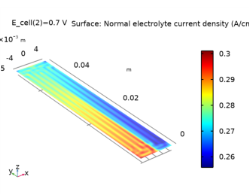
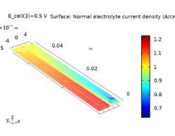
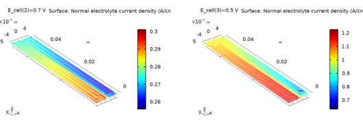
In the Settings window for Surface, click Replace Expression in the upper-right corner of the Expression section. From the menu, choose Component 1 (comp1)>Hydrogen Fuel Cell>fc.nIl - Normal electrolyte current density - A/m².
3
Locate the Expression section. In the Unit field, type A/cm^2.
Selection 1
1
Right-click Surface 1 and choose Selection.
2
In the Settings window for Selection, locate the Selection section.
3
From the Selection list, choose GDE, O2 Side.
O2 GDE Current Density
1
In the Model Builder window, click O2 GDE Current Density.
2
In the Settings window for 3D Plot Group, locate the Data section.
3
From the Parameter value (E_cell (V)) list, choose 0.7.
4
Locate the Plot Settings section. Clear the Plot dataset edges check box.
5
In the O2 GDE Current Density toolbar, click  Plot.
6
Locate the Data section. From the Parameter value (E_cell (V)) list, choose 0.5.
7
In the O2 GDE Current Density toolbar, click  Plot.
 
Appendix — Geometry Modeling Instructions
From the File menu, choose New.
New
In the New window, click  Model Wizard.
Model Wizard
1
In the Model Wizard window, click  3D.
2
Global Definitions
Parameters 1
1
In the Model Builder window, under Global Definitions click Parameters 1.
2
In the Settings window for Parameters, locate the Parameters section.
3
Click  Load from File.
4
Geometry 1
Work Plane 1 (wp1)
1
In the Geometry toolbar, click  Work Plane.
2
In the Settings window for Work Plane, locate the Plane Definition section.
3
In the z-coordinate text field, type H_gdl+H_mem/2.
Work Plane 1 (wp1)>Plane Geometry
In the Model Builder window, click Plane Geometry.
Work Plane 1 (wp1)>Rectangle 1 (r1)
1
In the Work Plane toolbar, click  Rectangle.
2
In the Settings window for Rectangle, locate the Size and Shape section.
3
In the Width text field, type W_ch.
4
In the Height text field, type W_plate-W_rib.
5
Locate the Position section. In the xw text field, type W_rib/2-N_ch*W_ribch.
6
In the yw text field, type W_rib/2.
7
Click  Build Selected.
8
Click the  Zoom Extents button in the Graphics toolbar.
Work Plane 1 (wp1)>Array 1 (arr1)
1
In the Work Plane toolbar, click  Transforms and choose Array.
2
3
In the Settings window for Array, locate the Size section.
4
In the xw size text field, type N_ch*2.
5
Locate the Displacement section. In the xw text field, type W_ribch.
6
Click  Build Selected.
Work Plane 1 (wp1)>Rectangle 2 (r2)
1
In the Work Plane toolbar, click  Rectangle.
2
In the Settings window for Rectangle, locate the Size and Shape section.
3
In the Width text field, type 2*N_ch*W_ribch.
4
In the Height text field, type W_ch.
5
Locate the Position section. In the xw text field, type -N_ch*W_ribch.
6
In the yw text field, type W_rib/2.
7
Click  Build Selected.
Work Plane 1 (wp1)>Array 2 (arr2)
1
In the Work Plane toolbar, click  Transforms and choose Array.
2
3
In the Settings window for Array, locate the Size section.
4
In the yw size text field, type N_ch.
5
Locate the Displacement section. In the yw text field, type W_ribch.
6
Click  Build Selected.
Work Plane 1 (wp1)>Mirror 1 (mir1)
1
In the Work Plane toolbar, click  Transforms and choose Mirror.
2
Select the objects arr2(1,1), arr2(1,2), and arr2(1,3) only.
3
In the Settings window for Mirror, locate the Input section.
4
Select the Keep input objects check box.
5
Locate the Point on Line of Reflection section. In the yw text field, type W_plate/2.
6
Locate the Normal Vector to Line of Reflection section. In the xw text field, type 0.
7
In the yw text field, type 1.
8
Click  Build Selected.
Work Plane 1 (wp1)>Square 1 (sq1)
1
In the Work Plane toolbar, click  Square.
2
In the Settings window for Square, locate the Size section.
3
In the Side length text field, type sqrt(2)*W_ribch*(N_ch+1).
4
Locate the Rotation Angle section. In the Rotation text field, type 45.
5
Click  Build Selected.
Work Plane 1 (wp1)>Square 2 (sq2)
1
In the Model Builder window, under Component 1 (comp1)>Geometry 1>Work Plane 1 (wp1)>Plane Geometry right-click Square 1 (sq1) and choose Duplicate.
2
In the Settings window for Square, locate the Rotation Angle section.
3
In the Rotation text field, type 45+90.
4
Click  Build Selected.
Work Plane 1 (wp1)>Square 3 (sq3)
1
Right-click Component 1 (comp1)>Geometry 1>Work Plane 1 (wp1)>Plane Geometry>Square 2 (sq2) and choose Duplicate.
2
In the Settings window for Square, locate the Rotation Angle section.
3
In the Rotation text field, type 45-90.
4
Click  Build Selected.
Work Plane 1 (wp1)>Copy 1 (copy1)
1
In the Work Plane toolbar, click  Transforms and choose Copy.
2
Select the objects sq1, sq2, and sq3 only.
3
In the Settings window for Copy, locate the Displacement section.
4
In the yw text field, type W_plate-(+W_ribch*(N_ch)).
5
Click  Build Selected.
6
Click the  Zoom Extents button in the Graphics toolbar.
Work Plane 1 (wp1)>Difference 1 (dif1)
1
In the Work Plane toolbar, click  Booleans and Partitions and choose Difference.
2
Select the objects arr2(1,1), arr2(1,2), and arr2(1,3) only.
3
In the Settings window for Difference, locate the Difference section.
4
Find the Objects to subtract subsection. Select the  Activate Selection toggle button.
5
6
Click  Build Selected.
Work Plane 1 (wp1)>Difference 2 (dif2)
1
In the Work Plane toolbar, click  Booleans and Partitions and choose Difference.
2
Select the objects mir1(1), mir1(2), and mir1(3) only.
3
In the Settings window for Difference, locate the Difference section.
4
Find the Objects to subtract subsection. Select the  Activate Selection toggle button.
5
Select the objects copy1(2) and copy1(3) only.
6
Click  Build Selected.
Work Plane 1 (wp1)>Difference 3 (dif3)
1
In the Work Plane toolbar, click  Booleans and Partitions and choose Difference.
2
Select the objects arr1(1,1), arr1(2,1), arr1(3,1), arr1(4,1), arr1(5,1), and arr1(6,1) only.
3
In the Settings window for Difference, locate the Difference section.
4
Find the Objects to subtract subsection. Select the  Activate Selection toggle button.
5
Select the objects copy1(1), sq2, and sq3 only.
6
Click  Build Selected.
Work Plane 1 (wp1)>Union 1 (uni1)
1
In the Work Plane toolbar, click  Booleans and Partitions and choose Union.
2
Click in the Graphics window and then press Ctrl+A to select all objects.
3
In the Settings window for Union, locate the Union section.
4
Clear the Keep interior boundaries check box.
5
Click  Build Selected.
Work Plane 1 (wp1)>Fillet 1 (fil1)
1
In the Work Plane toolbar, click  Fillet.
2
Click the  Zoom Box button in the Graphics toolbar.
3
On the object uni1, select Points 7, 10, 11, 14, 15, 18, 20, 21, 24, 25, 28, and 29 only.
4
In the Settings window for Fillet, locate the Radius section.
5
In the Radius text field, type r_ch.
6
Click  Build Selected.
Work Plane 1 (wp1)>Fillet 2 (fil2)
1
In the Work Plane toolbar, click  Fillet.
2
On the object fil1, select Points 10, 16, 22, 26, 32, and 38 only.
3
Click the  Zoom Out button in the Graphics toolbar.
4
Click the  Zoom Out button in the Graphics toolbar.
5
Click the  Zoom Box button in the Graphics toolbar.
6
On the object fil1, select Points 9, 10, 15, 16, 21, 22, 26, 29, 32, 35, 38, and 41 only.
7
In the Settings window for Fillet, locate the Radius section.
8
In the Radius text field, type W_ch+r_ch.
9
Click  Build Selected.
10
Click the  Zoom Extents button in the Graphics toolbar.
Channels
1
In the Model Builder window, right-click Geometry 1 and choose Extrude.
2
In the Settings window for Extrude, type Channels in the Label text field.
3
Locate the Distances section. In the table, enter the following settings:
4
Locate the Selections of Resulting Entities section. Select the Resulting objects selection check box.
5
From the Show in physics list, choose All levels.
6
Click  Build Selected.
Work Plane 2 (wp2)
1
In the Geometry toolbar, click  Work Plane.
2
In the Settings window for Work Plane, locate the Plane Definition section.
3
From the Plane list, choose zx-plane.
4
In the y-coordinate text field, type N_ch*W_ribch+W_ch.
5
Click  Build Selected.
Partition Domains 1 (pard1)
1
In the Geometry toolbar, click  Booleans and Partitions and choose Partition Domains.
2
In the Settings window for Partition Domains, locate the Partition Domains section.
3
From the Domains to partition list, choose Channels.
4
Click  Build Selected.
Work Plane 3 (wp3)
1
In the Geometry toolbar, click  Work Plane.
2
In the Settings window for Work Plane, locate the Plane Definition section.
3
From the Plane list, choose zx-plane.
4
In the y-coordinate text field, type W_plate-N_ch*W_ribch-W_ch.
5
Click  Build Selected.
Partition Domains 2 (pard2)
1
In the Geometry toolbar, click  Booleans and Partitions and choose Partition Domains.
2
In the Settings window for Partition Domains, locate the Partition Domains section.
3
From the Domains to partition list, choose Channels.
4
Click  Build Selected.
Channel Sweep Mesh Domains
1
In the Geometry toolbar, click  Selections and choose Box Selection.
2
In the Settings window for Box Selection, type Channel Sweep Mesh Domains in the Label text field.
3
Locate the Box Limits section. In the y minimum text field, type N_ch*W_ribch-W_ch.
4
In the y maximum text field, type W_plate-N_ch*W_ribch+W_ch.
5
Locate the Output Entities section. From the Include entity if list, choose Entity inside box.
6
Click  Build Selected.
Channel Tet Mesh Domains
1
In the Geometry toolbar, click  Selections and choose Difference Selection.
2
In the Settings window for Difference Selection, type Channel Tet Mesh Domains in the Label text field.
3
Locate the Input Entities section. Click  Add.
4
In the Add dialog box, select Channels in the Selections to add list.
5
6
In the Settings window for Difference Selection, locate the Input Entities section.
7
8
In the Add dialog box, select Channel Sweep Mesh Domains in the Selections to subtract list.
9
GDL
1
In the Geometry toolbar, click  Block.
2
In the Settings window for Block, type GDL in the Label text field.
3
Locate the Size and Shape section. In the Width text field, type 2*N_ch*W_ribch.
4
In the Depth text field, type W_plate.
5
In the Height text field, type H_gdl.
6
Locate the Position section. In the x text field, type -N_ch*W_ribch.
7
In the z text field, type H_mem/2.
8
Locate the Selections of Resulting Entities section. Select the Resulting objects selection check box.
9
Click  Build Selected.
Membrane
1
In the Geometry toolbar, click  Extrude.
2
In the Settings window for Extrude, type Membrane in the Label text field.
3
Locate the General section. From the Extrude from list, choose Faces.
4
On the object blk1, select Boundary 1 only.
5
From the Input object handling list, choose Keep.
6
Locate the Distances section. In the table, enter the following settings:
7
Locate the Selections of Resulting Entities section. Select the Resulting objects selection check box.
8
Click  Build Selected.
Union 1 (uni1)
1
In the Geometry toolbar, click  Booleans and Partitions and choose Union.
2
Click in the Graphics window and then press Ctrl+A to select all objects.
Rotate 1 (rot1)
1
In the Geometry toolbar, click  Transforms and choose Rotate.
2
3
In the Settings window for Rotate, locate the Input section.
4
Select the Keep input objects check box.
5
Locate the Rotation section. From the Axis type list, choose x-axis.
6
In the Angle text field, type 180.
7
Locate the Point on Axis of Rotation section. In the y text field, type W_plate/2.
8
Click  Build Selected.
H2 Side Domains
1
In the Geometry toolbar, click  Selections and choose Box Selection.
2
In the Settings window for Box Selection, type H2 Side Domains in the Label text field.
3
Locate the Box Limits section. In the z maximum text field, type -H_mem/4.
4
Click  Build Selected.
H2 Flow Channels
1
In the Geometry toolbar, click  Selections and choose Intersection Selection.
2
In the Settings window for Intersection Selection, type H2 Flow Channels in the Label text field.
3
Locate the Input Entities section. Click  Add.
4
In the Add dialog box, in the Selections to intersect list, choose Channels and H2 Side Domains.
5
6
In the Settings window for Intersection Selection, click  Build Selected.
Delete Entities 1 (del1)
1
Right-click Geometry 1 and choose Delete Entities.
2
In the Settings window for Delete Entities, locate the Entities or Objects to Delete section.
3
From the Geometric entity level list, choose Domain.
4
From the Selection list, choose H2 Flow Channels.
5
Click  Build Selected.
Upper GDL Boundary
1
In the Geometry toolbar, click  Selections and choose Box Selection.
2
In the Settings window for Box Selection, type Upper GDL Boundary in the Label text field.
3
Locate the Geometric Entity Level section. From the Level list, choose Boundary.
4
Locate the Box Limits section. In the z minimum text field, type H_gdl/2+H_mem/2.
5
In the z maximum text field, type H_gdl*3/2+H_mem.
6
Locate the Output Entities section. From the Include entity if list, choose Entity inside box.
O2 Current Collector
1
In the Geometry toolbar, click  Selections and choose Difference Selection.
2
In the Settings window for Difference Selection, type O2 Current Collector in the Label text field.
3
Locate the Geometric Entity Level section. From the Level list, choose Boundary.
4
Locate the Input Entities section. Click  Add.
5
In the Add dialog box, select Upper GDL Boundary in the Selections to add list.
6
7
In the Settings window for Difference Selection, locate the Input Entities section.
8
9
In the Add dialog box, select Channels in the Selections to subtract list.
10
Partition Faces 1 (parf1)
1
In the Geometry toolbar, click  Booleans and Partitions and choose Partition Faces.
2
In the Settings window for Partition Faces, locate the Partition Faces section.
3
From the Faces to partition list, choose O2 Current Collector.
4
From the Partition with list, choose Work plane.
5
Click  Build Selected.
Partition Faces 2 (parf2)
1
Right-click Partition Faces 1 (parf1) and choose Duplicate.
2
In the Settings window for Partition Faces, locate the Partition Faces section.
3
Find the Faces to partition subsection. Select the  Activate Selection toggle button.
4
From the Work plane list, choose Work Plane 2 (wp2).
5
Click  Build Selected.
Form Union (fin)
1
In the Model Builder window, under Component 1 (comp1)>Geometry 1 click Form Union (fin).
2
In the Settings window for Form Union/Assembly, locate the Form Union/Assembly section.
3
From the Action list, choose Form an assembly.
4
Click  Build Selected.
Inlets, O2 side
1
In the Geometry toolbar, click  Selections and choose Box Selection.
2
In the Settings window for Box Selection, type Inlets, O2 side in the Label text field.
3
Locate the Geometric Entity Level section. From the Level list, choose Boundary.
4
Locate the Box Limits section. In the x maximum text field, type -W_ribch*3+W_ch/10.
5
In the z minimum text field, type H_mem/2+H_gdl/2.
6
Locate the Output Entities section. From the Include entity if list, choose Entity inside box.
7
Click  Build Selected.
Outlets, O2 side
1
Right-click Inlets, O2 side and choose Duplicate.
2
In the Settings window for Box Selection, type Outlets, O2 side in the Label text field.
3
Locate the Box Limits section. In the x minimum text field, type W_ribch*3-W_ch/10.
4
In the x maximum text field, type Inf.
5
Click  Build Selected.
Slip Walls
1
In the Geometry toolbar, click  Selections and choose Difference Selection.
2
In the Settings window for Difference Selection, type Slip Walls in the Label text field.
3
Locate the Geometric Entity Level section. From the Level list, choose Boundary.
4
Locate the Input Entities section. Click  Add.
5
In the Add dialog box, select GDL in the Selections to add list.
6
7
In the Settings window for Difference Selection, locate the Input Entities section.
8
9
In the Add dialog box, select Channels in the Selections to subtract list.
10
Boundary Layer Walls
1
In the Geometry toolbar, click  Selections and choose Difference Selection.
2
In the Settings window for Difference Selection, type Boundary Layer Walls in the Label text field.
3
Locate the Geometric Entity Level section. From the Level list, choose Boundary.
4
Locate the Input Entities section. Click  Add.
5
In the Add dialog box, select Channels in the Selections to add list.
6
7
In the Settings window for Difference Selection, locate the Input Entities section.
8
9
In the Add dialog box, in the Selections to subtract list, choose Inlets, O2 side and Outlets, O2 side.
10
O2 Side Domains
1
In the Geometry toolbar, click  Selections and choose Box Selection.
2
In the Settings window for Box Selection, type O2 Side Domains in the Label text field.
3
Locate the Box Limits section. In the z minimum text field, type H_mem/4.
4
Click  Build Selected.
GDE, O2 Side
1
In the Geometry toolbar, click  Selections and choose Box Selection.
2
In the Settings window for Box Selection, type GDE, O2 Side in the Label text field.
3
Locate the Box Limits section. In the z minimum text field, type H_mem/4.
4
In the z maximum text field, type H_mem/2+H_gdl/2.
5
Locate the Output Entities section. From the Include entity if list, choose Entity inside box.
6
Locate the Geometric Entity Level section. From the Level list, choose Boundary.
GDE, H2 Side
1
Right-click GDE, O2 Side and choose Duplicate.
2
In the Settings window for Box Selection, type GDE, H2 Side in the Label text field.
3
Locate the Box Limits section. In the z minimum text field, type -H_mem/2-H_gdl/2.
4
In the z maximum text field, type -H_mem/4.
5
Click  Build Selected.
O2 Flow Channel
1
In the Geometry toolbar, click  Selections and choose Intersection Selection.
2
In the Settings window for Intersection Selection, type O2 Flow Channel in the Label text field.
3
Locate the Input Entities section. Click  Add.
4
In the Add dialog box, in the Selections to intersect list, choose Channels and O2 Side Domains.
5
H2 GDL
1
In the Geometry toolbar, click  Selections and choose Intersection Selection.
2
In the Settings window for Intersection Selection, type H2 GDL in the Label text field.
3
Locate the Input Entities section. Click  Add.
4
In the Add dialog box, in the Selections to intersect list, choose Channels and H2 Side Domains.
5
6
In the Settings window for Intersection Selection, locate the Input Entities section.
7
In the Selections to intersect list, select Channels.
8
Click  Delete.
9
10
In the Add dialog box, select GDL in the Selections to intersect list.
11
H2 GDL (intsel3)
1
In the Model Builder window, click H2 GDL.
2
In the Settings window for Intersection Selection, click  Build Selected.
O2 GDL
1
Right-click H2 GDL and choose Duplicate.
2
In the Settings window for Intersection Selection, type O2 GDL in the Label text field.
3
Locate the Input Entities section. In the Selections to intersect list, select H2 Side Domains.
4
Click  Delete.
5
6
In the Add dialog box, select O2 Side Domains in the Selections to intersect list.
7
8
In the Settings window for Intersection Selection, click  Build Selected.
O2 Flow Domains
1
In the Geometry toolbar, click  Selections and choose Union Selection.
2
In the Settings window for Union Selection, type O2 Flow Domains in the Label text field.
3
Locate the Input Entities section. Click  Add.
4
In the Add dialog box, in the Selections to add list, choose O2 Flow Channel and O2 GDL.
5
Lower GDL Boundary
1
In the Geometry toolbar, click  Selections and choose Box Selection.
2
In the Settings window for Box Selection, type Lower GDL Boundary in the Label text field.
3
Locate the Geometric Entity Level section. From the Level list, choose Boundary.
4
Locate the Box Limits section. In the z minimum text field, type -H_gdl*3/2-H_mem.
5
In the z maximum text field, type -H_gdl/2-H_mem/2.
6
Locate the Output Entities section. From the Include entity if list, choose Entity inside box.
7
Click  Build Selected.
Work Plane 1 (wp1)
In the Model Builder window, collapse the Component 1 (comp1)>Geometry 1>Work Plane 1 (wp1) node.
H2 Current Collector
1
In the Geometry toolbar, click  Selections and choose Difference Selection.
2
In the Settings window for Difference Selection, type H2 Current Collector in the Label text field.
3
Locate the Geometric Entity Level section. From the Level list, choose Boundary.
4
Locate the Input Entities section. Click  Add.
5
In the Add dialog box, select Lower GDL Boundary in the Selections to add list.
6
7
In the Settings window for Difference Selection, locate the Input Entities section.
8
9
In the Add dialog box, select Channels in the Selections to subtract list.
10
Channel Sweep Mesh Boundaries
1
In the Geometry toolbar, click  Selections and choose Adjacent Selection.
2
In the Settings window for Adjacent Selection, type Channel Sweep Mesh Boundaries in the Label text field.
3
Locate the Input Entities section. From the Geometric entity level list, choose Domain.
4
5
In the Add dialog box, select Channel Sweep Mesh Domains in the Input selections list.
6
Channel Tet Mesh Boundaries
1
Right-click Channel Sweep Mesh Boundaries and choose Duplicate.
2
In the Settings window for Adjacent Selection, type Channel Tet Mesh Boundaries in the Label text field.
3
Locate the Input Entities section. Click Build Preceding State.
4
In the Input selections list, select Channel Sweep Mesh Domains.
5
Click  Delete.
6
7
In the Add dialog box, select Channel Tet Mesh Domains in the Input selections list.
8
9
In the Settings window for Adjacent Selection, click  Build Selected.
Channel Mesh Sweep Faces
1
In the Geometry toolbar, click  Selections and choose Intersection Selection.
2
In the Settings window for Intersection Selection, locate the Geometric Entity Level section.
3
From the Level list, choose Boundary.
4
In the Label text field, type Channel Mesh Sweep Faces.
5
Locate the Input Entities section. Click  Add.
6
In the Add dialog box, in the Selections to intersect list, choose Channel Sweep Mesh Boundaries and Channel Tet Mesh Boundaries.
7
GDL Upper Boundary Mesh Sweep Area
1
In the Geometry toolbar, click  Selections and choose Box Selection.
2
In the Settings window for Box Selection, type GDL Upper Boundary Mesh Sweep Area in the Label text field.
3
Locate the Geometric Entity Level section. From the Level list, choose Boundary.
4
Locate the Box Limits section. In the y minimum text field, type N_ch*W_ribch+W_ch-W_ch/2.
5
In the y maximum text field, type W_plate-N_ch*W_ribch-W_ch+W_ch/2.
6
In the z minimum text field, type H_gdl/2+H_mem/2.
7
In the z maximum text field, type H_gdl*3/2+H_mem/2.
8
Locate the Output Entities section. From the Include entity if list, choose Entity inside box.
9
Click  Build Selected.
O2 Current Collector Mapped Mesh Boundaries
1
In the Geometry toolbar, click  Selections and choose Intersection Selection.
2
In the Settings window for Intersection Selection, type O2 Current Collector Mapped Mesh Boundaries in the Label text field.
3
Locate the Geometric Entity Level section. From the Level list, choose Boundary.
4
Locate the Input Entities section. Click  Add.
5
In the Add dialog box, in the Selections to intersect list, choose O2 Current Collector and GDL Upper Boundary Mesh Sweep Area.
6
O2 Current Collector Triangular Mesh Boundaries
1
In the Geometry toolbar, click  Selections and choose Difference Selection.
2
In the Settings window for Difference Selection, type O2 Current Collector Triangular Mesh Boundaries in the Label text field.
3
Locate the Geometric Entity Level section. From the Level list, choose Boundary.
4
Locate the Input Entities section. Click  Add.
5
In the Add dialog box, select O2 Current Collector in the Selections to add list.
6
7
In the Settings window for Difference Selection, locate the Input Entities section.
8
9
In the Add dialog box, select O2 Current Collector Mapped Mesh Boundaries in the Selections to subtract list.
10