PDF

Mass Transport Analysis of a High Temperature PEM Fuel Cell
Introduction
A high-temperature PEM based on phosphoric acid doped polymer membranes typically operates in a temperature window between 100°C and 200°C.
Water is produced on the cathode side due to the electrochemical reactions, but water may also be present on the anode side if the hydrogen fuel stream contains water. The latter may be the case if the hydrogen fuel stems from reforming of hydrocarbon fuels such as natural gas, alcohols or diesel.
Water build-up in the cell results in lower partial pressures of hydrogen and oxygen on the anode and cathode, respectively, and thereby also lowers the rate of the cell reactions.
The local water concentration in the cell may have a beneficial impact on the ion conductivity of the membrane, but if water condenses in the cell it may result in leaching of phosphoric acid out from the polymer matrix, irreversibly reducing the ion conducting capabilities of the membrane and the performance of the whole cell.
During normal operation above 100°C, water normally does not condensate in the cell, but knowledge about the water content in the porous electrodes during operation may also be desired in order to optimize shut-down procedures, since water may condensate when the temperature is lowered below 100°C.
This model example investigates the steady-state transport of reactants and water in a cell including both anode and cathode mass and momentum transport phenomena in the flow channels, gas diffusion layers (GDLs) and gas diffusion electrodes (GDEs), as well as electrochemical currents in the GDLs, the GDEs and the polymer membrane.
Model Definition
The geometry is shown in Figure 1.
Figure 1: Modeled geometry.
The following unknown variables are solved for in the model:
This is done by using a Hydrogen Fuel Cell interface, two Free and Porous Media Flow interfaces, along with Reacting Flow, H2 Gas Phase, and Reacting Flow, O2 Gas Phase multiphysics nodes.
Electrochemical currents
The Hydrogen Fuel Cell interface models the electrochemical currents using Ohm’s law, solving for in the GDLs, and in the GDEs, and in the membrane. In the GDEs the local current densities depend on the ionic and electronic potentials, but also on local reactant concentrations.
On the anode, hydrogen oxidation occurs according to
(no water molecules are assumed to be involved in the proton transport), and the following local current density expression is used for the hydrogen oxidation reaction:
where pH2 is the local hydrogen partial pressure and pref the reference pressure of 1 atm. is the overpotential with respect to the equilibrium potential of the reaction at atmospheric pressures of the reacting gases.
At the cathode, oxygen reacts together with the protons to form water according to
and the following current density expression is used for the oxygen reduction reaction:
where pO2 and pH2O are the local partial pressures of oxygen and water vapor, respectively.
The anode GDL boundaries facing the flow pattern ribs are set to zero electronic potential, and the corresponding boundaries at the cathode side are set to the cell potential. All other external boundaries are electrically isolating.
Mass transfer
The Hydrogen Fuel Cells interface also solves for the species mass fractions in the flow channels, the GDLs and the GDEs using the Maxwell-Stefan equations. Note that hydrogen and water species are present on the anode side whereas oxygen, water and nitrogen are present on the cathode side.
At the channel inlets mole fractions are specified, and outlet conditions are used at the channel outlets. All other external boundaries use zero flux conditions.
Momentum transfer
u and p are modeled by the compressible Navier-Stokes equations in the flow channels, and by the Brinkman equations in the GDLs and the GDEs, by using two Free and Porous Media Flow interfaces.
Couplings for the density, velocity, pressure and net mass sources and sinks are made to the Hydrogen Fuel Cell interface by using Reacting Flow, H2 Gas Phase and Reacting Flow, O2 Gas Phase multiphysics nodes.
At the flow channel inlet boundaries, laminar inlet flow velocity profiles are specified, whereas a pressure is specified at the flow channel outlet boundaries. To model a multiple parallel channel configuration, symmetry boundary conditions are applied along the long sides of the GDLs and the GDEs. All other wall boundaries use no slip conditions.
Results and Discussion
Figure 2 shows the polarization plot of the cell.
Figure 2: Polarization plot.
Figure 3 shows the ionic current in the z direction at the center of the membrane for 0.4 V. In the y direction the current density is lower toward the outlet (due to lower reactant concentrations).In the x direction the currents density is highest in the region close to the channel, where the reactant concentrations are higher, but the current density is reduced toward the very center of the channel. This is due to ohmic drops in the GDLs.
Figure 3: Ionic current in the polymer membrane at 0.4 V.
Figure 4 shows the hydrogen and oxygen mole fractions for the same voltage level. The oxygen mole fraction is significantly lower in the porous electrode and toward the end of the flow channel compared to the inlet level. For the anode the trend is the same but the hydrogen mole fraction level is more uniform.
Figure 4: Hydrogen mole fraction at the anode (top) and oxygen mole fraction at the cathode (bottom) in the cell at 0.4 V.
Figure 5 shows the water mole fraction in the cell for the same voltage level. The mole fraction increase due to water production at the cathode is much larger than the effect of removing hydrogen from the gas stream at the anode for these flow and current levels.
Figure 5: Water mole fraction on the anode and cathode side in the cell at 0.4 V.
Reference
1. E.U. Ubong, Z. Shi, and X. Wang, “Three-Dimensional Modeling and Experimental Study of a High Temperature PBI-Based PEM Fuel Cell,” J. Electrochemical Soc., vol. 156, no. 10, pp. B1276–B1282, 2009.
Application Library path: Fuel_Cell_and_Electrolyzer_Module/Fuel_Cells/ht_pem
Modeling Instructions
From the File menu, choose New.
New
In the New window, click  Model Wizard.
Model Wizard
1
In the Model Wizard window, click  3D.
2
In the Select Physics tree, select Electrochemistry>Hydrogen Fuel Cells>Proton Exchange (fc).
3
Click Add.
4
In the Select Physics tree, select Fluid Flow>Porous Media and Subsurface Flow>Free and Porous Media Flow (fp).
5
Click Add.
6
In the Velocity field text field, type ua.
7
In the Velocity field components table, enter the following settings:
8
In the Pressure text field, type pa.
9
In the Select Physics tree, select Fluid Flow>Porous Media and Subsurface Flow>Free and Porous Media Flow (fp).
10
Click Add.
11
In the Velocity field text field, type uc.
12
In the Velocity field components table, enter the following settings:
13
In the Pressure text field, type pc.
14
Click  Study.
15
In the Select Study tree, select Preset Studies for Selected Physics Interfaces>Hydrogen Fuel Cell>Stationary with Initialization.
16
Global Definitions
Load the model parameters from a text file.
Parameters 1
1
In the Model Builder window, under Global Definitions click Parameters 1.
2
In the Settings window for Parameters, locate the Parameters section.
3
Click  Load from File.
4
Geometry 1
Draw the channels, gas diffusion layers, porous gas diffusion electrodes and membrane using rectangular blocks.
Anode Channel
1
In the Geometry toolbar, click  Block.
2
In the Settings window for Block, type Anode Channel in the Label text field.
3
Locate the Size and Shape section. In the Width text field, type W_ch.
4
In the Depth text field, type L.
5
In the Height text field, type H_ch.
6
Locate the Position section. In the x text field, type W_rib/2.
7
Locate the Selections of Resulting Entities section. Select the Resulting objects selection check box.
8
Click  Build Selected.
Anode GDL
1
Right-click Anode Channel and choose Duplicate.
2
In the Settings window for Block, type Anode GDL in the Label text field.
3
Locate the Size and Shape section. In the Width text field, type (W_ch+W_rib).
4
In the Height text field, type H_gdl.
5
Locate the Position section. In the x text field, type 0.
6
In the z text field, type H_ch.
7
Click  Build Selected.
Anode GDE
1
Right-click Anode GDL and choose Duplicate.
2
In the Settings window for Block, type Anode GDE in the Label text field.
3
Locate the Size and Shape section. In the Height text field, type H_electrode.
4
Locate the Position section. In the z text field, type H_ch+H_gdl.
5
Click  Build Selected.
Membrane
1
Right-click Anode GDE and choose Duplicate.
2
In the Settings window for Block, type Membrane in the Label text field.
3
Locate the Size and Shape section. In the Height text field, type H_membrane.
4
Locate the Position section. In the z text field, type H_ch+H_gdl+H_electrode.
5
Click  Build Selected.
Cathode GDE
1
Right-click Membrane and choose Duplicate.
2
In the Settings window for Block, type Cathode GDE in the Label text field.
3
Locate the Size and Shape section. In the Width text field, type W_ch+W_rib.
4
In the Height text field, type H_electrode.
5
Locate the Position section. In the z text field, type H_ch+H_gdl+H_electrode+H_membrane.
6
Click  Build Selected.
Cathode GDL
1
Right-click Cathode GDE and choose Duplicate.
2
In the Settings window for Block, type Cathode GDL in the Label text field.
3
Locate the Size and Shape section. In the Height text field, type H_gdl.
4
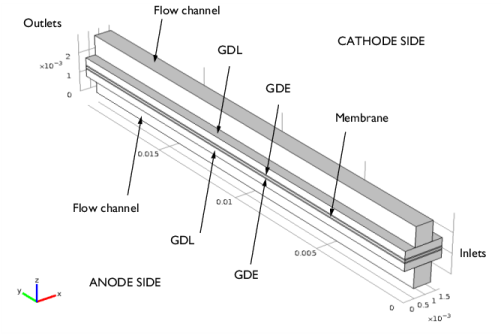
Locate the Position section. In the z text field, type H_ch+H_gdl+H_electrode+H_membrane+H_electrode.
5
Click  Build Selected.
Cathode Channel
1
Right-click Cathode GDL and choose Duplicate.
2
In the Settings window for Block, type Cathode Channel in the Label text field.
3
Locate the Size and Shape section. In the Width text field, type W_ch.
4
In the Height text field, type H_ch.
5
Locate the Position section. In the x text field, type W_rib/2.
6
In the z text field, type H_ch+H_gdl+H_electrode+H_membrane+H_electrode+H_gdl.
7
Click  Build All Objects.
Definitions
Now create some additional selections of certain parts of the geometry to facilitate setting up the physics later on.
Anode Inlet
1
In the Definitions toolbar, click  Explicit.
2
In the Settings window for Explicit, type Anode Inlet in the Label text field.
3
Locate the Input Entities section. From the Geometric entity level list, choose Boundary.
4
Cathode Inlet
1
In the Definitions toolbar, click  Explicit.
2
In the Settings window for Explicit, type Cathode Inlet in the Label text field.
3
Locate the Input Entities section. From the Geometric entity level list, choose Boundary.
4
Anode Outlet
1
In the Definitions toolbar, click  Explicit.
2
In the Settings window for Explicit, type Anode Outlet in the Label text field.
3
Locate the Input Entities section. From the Geometric entity level list, choose Boundary.
4
Cathode Outlet
1
In the Definitions toolbar, click  Explicit.
2
In the Settings window for Explicit, type Cathode Outlet in the Label text field.
3
Locate the Input Entities section. From the Geometric entity level list, choose Boundary.
4
Anode Compartment
1
In the Definitions toolbar, click  Union.
2
In the Settings window for Union, type Anode Compartment in the Label text field.
3
Locate the Input Entities section. Under Selections to add, click  Add.
4
In the Add dialog box, in the Selections to add list, choose Anode Channel, Anode GDL, and Anode GDE.
5
Cathode Compartment
1
In the Definitions toolbar, click  Union.
2
In the Settings window for Union, type Cathode Compartment in the Label text field.
3
Locate the Input Entities section. Under Selections to add, click  Add.
4
In the Add dialog box, in the Selections to add list, choose Cathode GDE, Cathode GDL, and Cathode Channel.
5
Free and Porous Media Flow- Anode
Set up the domains applicable for the flow interfaces.
1
In the Model Builder window, under Component 1 (comp1) click Free and Porous Media Flow (fp).
2
In the Settings window for Free and Porous Media Flow, type Free and Porous Media Flow- Anode in the Label text field.
3
Locate the Domain Selection section. From the Selection list, choose Anode Compartment.
Free and Porous Media Flow - Cathode
1
In the Model Builder window, under Component 1 (comp1) click Free and Porous Media Flow 2 (fp2).
2
In the Settings window for Free and Porous Media Flow, type Free and Porous Media Flow - Cathode in the Label text field.
3
Locate the Domain Selection section. From the Selection list, choose Cathode Compartment.
Multiphysics
Next, couple the interfaces appropriately using the reacting flow multiphysics coupling nodes. Note that currently, the multiphysics nodes may not be applicable to any domain selections, but the selections will be automatically updated when the Hydrogen Fuel Cell interface is set up.
Reacting Flow, H2 Gas Phase 1 (rfh1)
In the Physics toolbar, click  Multiphysics Couplings and choose Domain>Reacting Flow, H2 Gas Phase.
Reacting Flow, O2 Gas Phase 1 (rfo1)
1
In the Physics toolbar, click  Multiphysics Couplings and choose Domain>Reacting Flow, O2 Gas Phase.
2
In the Settings window for Reacting Flow, O2 Gas Phase, locate the Coupled Interfaces section.
3
From the Fluid flow list, choose Free and Porous Media Flow - Cathode (fp2).
Hydrogen Fuel Cell (fc)
Set up the current distribution and mass transport model. The default gas species are hydrogen and water on the anode side, and oxygen, nitrogen and water on the cathode side. Start with adding the relevant domain nodes.
1
In the Model Builder window, under Component 1 (comp1) click Hydrogen Fuel Cell (fc).
Membrane 1
1
In the Physics toolbar, click  Domains and choose Membrane.
2
In the Settings window for Membrane, locate the Domain Selection section.
3
From the Selection list, choose Membrane.
H2 Gas Diffusion Electrode 1
1
In the Physics toolbar, click  Domains and choose H2 Gas Diffusion Electrode.
2
In the Settings window for H2 Gas Diffusion Electrode, locate the Domain Selection section.
3
From the Selection list, choose Anode GDE.
H2 Gas Diffusion Layer 1
1
In the Physics toolbar, click  Domains and choose H2 Gas Diffusion Layer.
2
In the Settings window for H2 Gas Diffusion Layer, locate the Domain Selection section.
3
From the Selection list, choose Anode GDL.
H2 Flow Channel 1
1
In the Physics toolbar, click  Domains and choose H2 Flow Channel.
2
In the Settings window for H2 Flow Channel, locate the Domain Selection section.
3
From the Selection list, choose Anode Channel.
O2 Gas Diffusion Electrode 1
1
In the Physics toolbar, click  Domains and choose O2 Gas Diffusion Electrode.
2
In the Settings window for O2 Gas Diffusion Electrode, locate the Domain Selection section.
3
From the Selection list, choose Cathode GDE.
O2 Gas Diffusion Layer 1
1
In the Physics toolbar, click  Domains and choose O2 Gas Diffusion Layer.
2
In the Settings window for O2 Gas Diffusion Layer, locate the Domain Selection section.
3
From the Selection list, choose Cathode GDL.
O2 Flow Channel 1
1
In the Physics toolbar, click  Domains and choose O2 Flow Channel.
2
In the Settings window for O2 Flow Channel, locate the Domain Selection section.
3
From the Selection list, choose Cathode Channel.
Electrolyte Phase 1
Set up the electrolyte conductivity in the Electrolyte Phase node. Note that in the H2 Gas Phase and O2 Gas Phase nodes, the settings are either the default option or automatically set by the multiphysics coupling nodes.
1
In the Model Builder window, click Electrolyte Phase 1.
2
In the Settings window for Electrolyte Phase, locate the Electrolyte Charge Transport section.
3
In the σl text field, type sigma_m.
H2 Gas Diffusion Electrode 1
Set up the properties of the H2 Gas Diffusion Electrode node. The details of electrode kinetics are set in the child node. Note that the reference equilibrium potential is calculated automatically when the default Built in option is used.
1
In the Model Builder window, click H2 Gas Diffusion Electrode 1.
2
In the Settings window for H2 Gas Diffusion Electrode, locate the Electrode Charge Transport section.
3
In the σs text field, type sigma_gdl.
4
Locate the Effective Electrolyte Charge Transport section. In the εl text field, type eps_l.
5
Locate the Gas Transport section. In the εg text field, type eps_cl.
H2 Gas Diffusion Electrode Reaction 1
1
In the Model Builder window, expand the H2 Gas Diffusion Electrode 1 node, then click H2 Gas Diffusion Electrode Reaction 1.
2
In the Settings window for H2 Gas Diffusion Electrode Reaction, locate the Electrode Kinetics section.
3
In the i0,ref(T) text field, type i0_ref_a.
4
Locate the Active Specific Surface Area section. In the av text field, type Av.
H2 Gas Diffusion Layer 1
Set up the properties of the H2 Gas Diffusion Layer node.
1
In the Model Builder window, click H2 Gas Diffusion Layer 1.
2
In the Settings window for H2 Gas Diffusion Layer, locate the Electrode Charge Transport section.
3
In the σs text field, type sigma_gdl.
4
Locate the Gas Transport section. In the εg text field, type eps_gdl.
O2 Gas Diffusion Electrode 1
Set up the properties of the O2 Gas Diffusion Electrode node. The details of electrode kinetics are set in the child node. Note that the reference equilibrium potential is calculated automatically when the default Built in option is used.
1
In the Model Builder window, click O2 Gas Diffusion Electrode 1.
2
In the Settings window for O2 Gas Diffusion Electrode, locate the Electrode Charge Transport section.
3
In the σs text field, type sigma_gdl.
4
Locate the Effective Electrolyte Charge Transport section. In the εl text field, type eps_l.
5
Locate the Gas Transport section. In the εg text field, type eps_cl.
O2 Gas Diffusion Electrode Reaction 1
1
In the Model Builder window, expand the O2 Gas Diffusion Electrode 1 node, then click O2 Gas Diffusion Electrode Reaction 1.
2
In the Settings window for O2 Gas Diffusion Electrode Reaction, locate the Electrode Kinetics section.
3
In the i0,ref(T) text field, type i0_ref_c.
4
In the αa text field, type 4-alpha_c.
5
Locate the Active Specific Surface Area section. In the av text field, type Av.
O2 Gas Diffusion Layer 1
Set up the properties of the O2 Gas Diffusion Layer node.
1
In the Model Builder window, click O2 Gas Diffusion Layer 1.
2
In the Settings window for O2 Gas Diffusion Layer, locate the Electrode Charge Transport section.
3
In the σs text field, type sigma_gdl.
4
Locate the Gas Transport section. In the εg text field, type eps_gdl.
There are no settings required on the flow channel nodes, other than the domain selection. Next, set up the boundary conditions and initial values.
Electronic Conducting Phase 1
In the Model Builder window, click Electronic Conducting Phase 1.
Electric Ground 1
1
In the Physics toolbar, click  Attributes and choose Electric Ground.
2
Electronic Conducting Phase 1
In the Model Builder window, click Electronic Conducting Phase 1.
Electric Potential 1
1
In the Physics toolbar, click  Attributes and choose Electric Potential.
2
3
In the Settings window for Electric Potential, locate the Electric Potential section.
4
In the φs,bnd text field, type V_cell.
Initial Values 1
1
In the Model Builder window, expand the Component 1 (comp1)>Hydrogen Fuel Cell (fc)>H2 Gas Phase 1 node, then click Initial Values 1.
2
In the Settings window for Initial Values, locate the Initial Values section.
3
In the x0,H2O text field, type x_H2O_in.
H2 Gas Phase 1
In the Model Builder window, click H2 Gas Phase 1.
H2 Inlet 1
1
In the Physics toolbar, click  Attributes and choose H2 Inlet.
2
In the Settings window for H2 Inlet, locate the Boundary Selection section.
3
From the Selection list, choose Anode Inlet.
4
Locate the Mixture Specification section. In the x0,H2O text field, type x_H2O_in.
H2 Gas Phase 1
In the Model Builder window, click H2 Gas Phase 1.
H2 Outlet 1
1
In the Physics toolbar, click  Attributes and choose H2 Outlet.
2
In the Settings window for H2 Outlet, locate the Boundary Selection section.
3
From the Selection list, choose Anode Outlet.
Initial Values 1
1
In the Model Builder window, expand the Component 1 (comp1)>Hydrogen Fuel Cell (fc)>O2 Gas Phase 1 node, then click Initial Values 1.
2
In the Settings window for Initial Values, locate the Initial Values section.
3
In the x0,H2O text field, type x_H2O_in.
4
In the x0,N2 text field, type x_N2_in.
O2 Gas Phase 1
In the Model Builder window, click O2 Gas Phase 1.
O2 Inlet 1
1
In the Physics toolbar, click  Attributes and choose O2 Inlet.
2
In the Settings window for O2 Inlet, locate the Boundary Selection section.
3
From the Selection list, choose Cathode Inlet.
4
Locate the Mixture Specification section. In the x0,H2O text field, type x_H2O_in.
5
In the x0,N2 text field, type x_N2_in.
O2 Gas Phase 1
In the Model Builder window, click O2 Gas Phase 1.
O2 Outlet 1
1
In the Physics toolbar, click  Attributes and choose O2 Outlet.
2
In the Settings window for O2 Outlet, locate the Boundary Selection section.
3
From the Selection list, choose Cathode Outlet.
Free and Porous Media Flow- Anode (fp)
Next, set up the fluid flow model on the anode side. Note that the flow is compressible.
1
In the Model Builder window, under Component 1 (comp1) click Free and Porous Media Flow- Anode (fp).
2
In the Settings window for Free and Porous Media Flow, locate the Physical Model section.
3
From the Compressibility list, choose Compressible flow (Ma<0.3).
Define the pressure reference level in the interface properties.
4
In the pref text field, type p_ref.
Set up the properties of the porous gas diffusion electrode, gas diffusion layer and the flow channel. Note that the density and viscosity of the gas mixture are calculated by the Hydrogen Fuel Cell interface and automatically set by the multiphysics coupling nodes.
Fluid and Matrix Properties 1
1
In the Physics toolbar, click  Domains and choose Fluid and Matrix Properties.
2
In the Settings window for Fluid and Matrix Properties, locate the Domain Selection section.
3
From the Selection list, choose Anode GDL.
4
Locate the Porous Matrix Properties section. From the εp list, choose User defined. In the associated text field, type eps_gdl.
5
From the κ list, choose User defined. In the associated text field, type kappa_gdl.
Fluid and Matrix Properties 2
1
In the Physics toolbar, click  Domains and choose Fluid and Matrix Properties.
2
In the Settings window for Fluid and Matrix Properties, locate the Domain Selection section.
3
From the Selection list, choose Anode GDE.
4
Locate the Porous Matrix Properties section. From the εp list, choose User defined. In the associated text field, type eps_cl.
5
From the κ list, choose User defined. In the associated text field, type kappa_cl.
Wall 1
1
Click the  Show More Options button in the Model Builder toolbar.
2
In the Show More Options dialog box, in the tree, select the check box for the node Physics>Advanced Physics Options.
3
4
In the Model Builder window, click Wall 1.
5
In the Settings window for Wall, click to expand the Constraint Settings section.
6
From the Apply reaction terms on list, choose All physics (symmetric).
Inlet 1
Now set up the inlet and outlet conditions on the corresponding boundaries.
1
In the Physics toolbar, click  Boundaries and choose Inlet.
2
In the Settings window for Inlet, locate the Boundary Selection section.
3
From the Selection list, choose Anode Inlet.
4
Locate the Boundary Condition section. From the list, choose Fully developed flow.
5
Locate the Fully Developed Flow section. In the Uav text field, type U_in_anode.
Outlet 1
1
In the Physics toolbar, click  Boundaries and choose Outlet.
2
In the Settings window for Outlet, locate the Boundary Selection section.
3
From the Selection list, choose Anode Outlet.
4
Locate the Pressure Conditions section. Select the Normal flow check box.
5
Click to expand the Constraint Settings section.
Symmetry 1
1
In the Physics toolbar, click  Boundaries and choose Symmetry.
2
Free and Porous Media Flow - Cathode (fp2)
Set up the fluid flow model on the cathode side in the same way.
1
In the Model Builder window, under Component 1 (comp1) click Free and Porous Media Flow - Cathode (fp2).
2
In the Settings window for Free and Porous Media Flow, locate the Physical Model section.
3
From the Compressibility list, choose Compressible flow (Ma<0.3).
Define the pressure reference level in the interface properties.
4
In the pref text field, type p_ref.
Fluid and Matrix Properties 1
1
In the Physics toolbar, click  Domains and choose Fluid and Matrix Properties.
2
In the Settings window for Fluid and Matrix Properties, locate the Domain Selection section.
3
From the Selection list, choose Cathode GDL.
4
Locate the Porous Matrix Properties section. From the εp list, choose User defined. In the associated text field, type eps_gdl.
5
From the κ list, choose User defined. In the associated text field, type kappa_gdl.
Fluid and Matrix Properties 2
1
In the Physics toolbar, click  Domains and choose Fluid and Matrix Properties.
2
In the Settings window for Fluid and Matrix Properties, locate the Domain Selection section.
3
From the Selection list, choose Cathode GDE.
4
Locate the Porous Matrix Properties section. From the εp list, choose User defined. In the associated text field, type eps_cl.
5
From the κ list, choose User defined. In the associated text field, type kappa_cl.
Wall 1
1
In the Model Builder window, click Wall 1.
2
In the Settings window for Wall, locate the Constraint Settings section.
3
From the Apply reaction terms on list, choose All physics (symmetric).
Symmetry 1
1
In the Physics toolbar, click  Boundaries and choose Symmetry.
2
Inlet 1
1
In the Physics toolbar, click  Boundaries and choose Inlet.
2
In the Settings window for Inlet, locate the Boundary Selection section.
3
From the Selection list, choose Cathode Inlet.
4
Locate the Boundary Condition section. From the list, choose Fully developed flow.
5
Locate the Fully Developed Flow section. In the Uav text field, type U_in_cathode.
Outlet 1
1
In the Physics toolbar, click  Boundaries and choose Outlet.
2
In the Settings window for Outlet, locate the Boundary Selection section.
3
From the Selection list, choose Cathode Outlet.
4
Locate the Pressure Conditions section. Select the Normal flow check box.
Global Definitions
Default Model Inputs
Use the Default Model Inputs node to set the Temperature for the entire model. This node may be accessed by multiple physics nodes.
1
In the Model Builder window, under Global Definitions click Default Model Inputs.
2
In the Settings window for Default Model Inputs, locate the Browse Model Inputs section.
3
In the tree, select General>Temperature (K) - minput.T.
4
Find the Expression for remaining selection subsection. In the Temperature text field, type T.
Mesh 1
First create a mapped 2D mesh in the plane normal to the channel direction, then sweep this mesh in the channel direction.
Edge 1
1
In the Mesh toolbar, click  Boundary and choose Edge.
2
Size 1
1
Right-click Edge 1 and choose Size.
2
In the Settings window for Size, locate the Element Size section.
3
Click the Custom button.
4
Locate the Element Size Parameters section. Select the Maximum element size check box.
5
Edge 2
1
In the Mesh toolbar, click  Boundary and choose Edge.
2
Distribution 1
1
Right-click Edge 2 and choose Distribution.
2
In the Settings window for Distribution, locate the Distribution section.
3
From the Distribution type list, choose Predefined.
4
In the Number of elements text field, type 8.
5
In the Element ratio text field, type 4.
Edge 3
1
In the Model Builder window, under Component 1 (comp1)>Mesh 1 right-click Edge 2 and choose Duplicate.
2
In the Settings window for Edge, locate the Edge Selection section.
3
Click  Clear Selection.
4
Distribution 1
1
In the Model Builder window, expand the Edge 3 node, then click Distribution 1.
2
In the Settings window for Distribution, locate the Distribution section.
3
Select the Reverse direction check box.
Edge 4
1
In the Mesh toolbar, click  Boundary and choose Edge.
2
Distribution 1
1
Right-click Edge 4 and choose Distribution.
2
In the Settings window for Distribution, locate the Distribution section.
3
In the Number of elements text field, type 6.
Edge 5
1
In the Mesh toolbar, click  Boundary and choose Edge.
2
Distribution 1
1
Right-click Edge 5 and choose Distribution.
Larger concentration gradients are expected in the cathode catalyst layer (due to the lower diffusion coefficient of oxygen), therefore use a higher element density in the cathode.
2
In the Settings window for Distribution, locate the Distribution section.
3
In the Number of elements text field, type 10.
Edge 6
1
In the Mesh toolbar, click  Boundary and choose Edge.
2
Distribution 1
1
Right-click Edge 6 and choose Distribution.
2
In the Settings window for Distribution, locate the Distribution section.
3
In the Number of elements text field, type 3.
Edge 7
1
In the Mesh toolbar, click  Boundary and choose Edge.
2
Distribution 1
1
Right-click Edge 7 and choose Distribution.
2
In the Settings window for Distribution, locate the Distribution section.
3
From the Distribution type list, choose Predefined.
4
In the Number of elements text field, type 8.
5
In the Element ratio text field, type 2.
6
Select the Symmetric distribution check box.
Mapped 1
1
In the Mesh toolbar, click  Boundary and choose Mapped.
2
Swept 1
In the Mesh toolbar, click  Swept.
Size 1
1
Right-click Swept 1 and choose Size.
2
In the Settings window for Size, locate the Element Size section.
3
Click the Custom button.
4
Locate the Element Size Parameters section. Select the Maximum element size check box.
5
6
Click  Build Selected.
Definitions
Add a domain probe for the integral of the electrochemical current density to get a polarization plot automatically during the parametric solver process. You can then use this probe also for creating a polarization curve during postprocessing.
Domain Probe 1 (dom1)
1
In the Definitions toolbar, click  Probes and choose Domain Probe.
2
In the Settings window for Domain Probe, locate the Probe Type section.
3
From the Type list, choose Integral.
4
Locate the Source Selection section. From the Selection list, choose Anode GDE.
5
Locate the Expression section. In the Expression text field, type fc.iv_h2gder1/((W_ch+W_rib)*L)/1e4.
Study 1
The problem is now ready for solving. Firstly, solve for current distribution initialization (both primary and secondary) in two study steps, followed by flow in two subsequent study steps. Finally, solve the entire model including the multiphysics couplings in the final step, along with an auxiliary sweep to solve for a range of potentials and simulate a polarization plot.
Step 1: Current Distribution Initialization
1
In the Model Builder window, under Study 1 click Step 1: Current Distribution Initialization.
2
In the Settings window for Current Distribution Initialization, locate the Physics and Variables Selection section.
3
In the table, clear the Solve for check boxes for Free and Porous Media Flow- Anode (fp) and Free and Porous Media Flow - Cathode (fp2).
4
In the table, clear the Solve for check boxes for Reacting Flow, H2 Gas Phase 1 (rfh1) and Reacting Flow, O2 Gas Phase 1 (rfo1).
Current Distribution Initialization 2
1
In the Study toolbar, click  Study Steps and choose Other>Current Distribution Initialization.
2
In the Settings window for Current Distribution Initialization, locate the Study Settings section.
3
From the Current distribution type list, choose Secondary.
4
Locate the Physics and Variables Selection section. In the table, clear the Solve for check boxes for Free and Porous Media Flow- Anode (fp) and Free and Porous Media Flow - Cathode (fp2).
5
In the table, clear the Solve for check boxes for Reacting Flow, H2 Gas Phase 1 (rfh1) and Reacting Flow, O2 Gas Phase 1 (rfo1).
Step 3: Stationary
1
In the Model Builder window, click Step 3: Stationary.
2
In the Settings window for Stationary, locate the Physics and Variables Selection section.
3
In the table, clear the Solve for check boxes for Hydrogen Fuel Cell (fc) and Free and Porous Media Flow - Cathode (fp2).
4
In the table, clear the Solve for check boxes for Reacting Flow, H2 Gas Phase 1 (rfh1) and Reacting Flow, O2 Gas Phase 1 (rfo1).
Stationary 2
1
In the Study toolbar, click  Study Steps and choose Stationary>Stationary.
2
In the Settings window for Stationary, locate the Physics and Variables Selection section.
3
In the table, clear the Solve for check boxes for Hydrogen Fuel Cell (fc) and Free and Porous Media Flow- Anode (fp).
4
In the table, clear the Solve for check boxes for Reacting Flow, H2 Gas Phase 1 (rfh1) and Reacting Flow, O2 Gas Phase 1 (rfo1).
Stationary 3
1
In the Study toolbar, click  Study Steps and choose Stationary>Stationary.
2
In the Settings window for Stationary, click to expand the Study Extensions section.
3
Select the Auxiliary sweep check box.
4
Use the range operator to create a list of potentials from 0.95 to 0.4 V, using steps -50 mV for the first steps, and then -100 mV toward the end.
5
6
In the Study toolbar, click  Compute.
Results
Several default plots are generated. Among them are the plots seen in Figure 4 and Figure 5 that show the hydrogen, oxygen and water mole fraction distributions.
Polarization Plot
Modify the probe plot as follows to reproduce the polarization plot in Figure 2.
1
In the Model Builder window, expand the Results>Probe Plot Group 15 node, then click Probe Plot Group 15.
2
In the Settings window for 1D Plot Group, type Polarization Plot in the Label text field.
3
Click to expand the Title section. From the Title type list, choose Label.
4
Locate the Plot Settings section. Select the x-axis label check box.
5
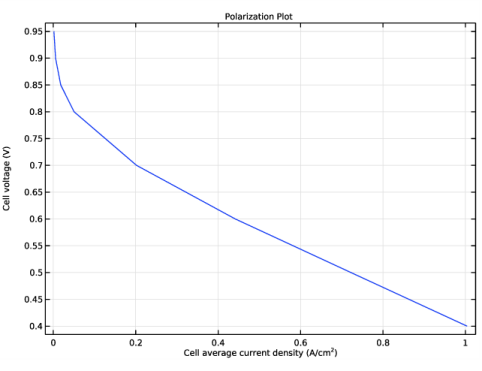
In the associated text field, type Cell average current density (A/cm<sup>2</sup>).
6
Select the y-axis label check box.
7
8
Select the Flip the x- and y-axes check box.
9
Locate the Legend section. Clear the Show legends check box.
10
In the Polarization Plot toolbar, click  Plot.
11
Click the  Zoom Extents button in the Graphics toolbar.
Cut Plane 1
Next, reproduce the ionic current plot of Figure 3. Begin by creating a Cut Plane dataset.
1
In the Results toolbar, click  Cut Plane.
2
In the Settings window for Cut Plane, locate the Plane Data section.
3
From the Plane list, choose xy-planes.
4
In the z-coordinate text field, type H_ch+H_gdl+H_electrode+H_membrane/2.
2D Plot Group 16
1
In the Results toolbar, click  2D Plot Group.
2
In the Settings window for 2D Plot Group, locate the Data section.
3
From the Dataset list, choose Cut Plane 1.
Contour 1
1
Right-click 2D Plot Group 16 and choose Contour.
2
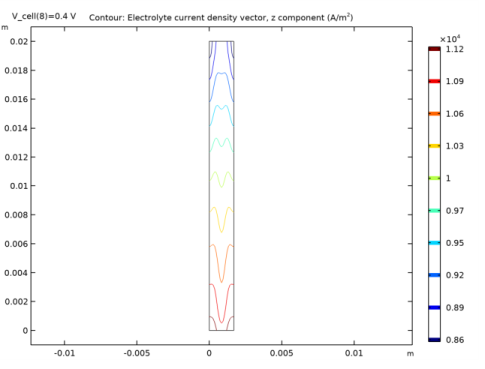
In the Settings window for Contour, click Replace Expression in the upper-right corner of the Expression section. From the menu, choose Component 1 (comp1)>Hydrogen Fuel Cell>Electrolyte current density vector - A/m²>fc.Ilz - Electrolyte current density vector, z component.
3
Locate the Levels section. In the Total levels text field, type 10.
Membrane Current Density
1
In the Model Builder window, click 2D Plot Group 16.
2
In the 2D Plot Group 16 toolbar, click  Plot.
3
Click the  Zoom Extents button in the Graphics toolbar.
4
In the Settings window for 2D Plot Group, type Membrane Current Density in the Label text field.