|
|
|
|
•
|
|
•
|
|
-
|
|
-
|
b = -0.097
|
|
-
|
|
-
|
c = -0.60
|
|
1
|
|
2
|
|
3
|
Click Add.
|
|
4
|
Click
|
|
5
|
|
6
|
Click
|
|
1
|
|
2
|
|
3
|
|
1
|
|
2
|
|
3
|
|
4
|
|
1
|
|
2
|
|
3
|
|
1
|
|
2
|
Select the object cyl1 only.
|
|
3
|
|
4
|
|
5
|
Select the object cyl2 only.
|
|
6
|
|
1
|
|
2
|
|
3
|
|
4
|
|
5
|
|
6
|
|
7
|
|
8
|
|
1
|
|
2
|
Select the object dif1 only.
|
|
3
|
|
4
|
|
5
|
Select the object cyl3 only.
|
|
6
|
|
1
|
|
2
|
|
3
|
|
4
|
|
5
|
|
6
|
|
1
|
|
2
|
Click in the Graphics window and then press Ctrl+A to select both objects.
|
|
3
|
|
4
|
|
1
|
|
2
|
|
3
|
|
4
|
|
5
|
|
6
|
|
7
|
|
8
|
|
1
|
|
2
|
Click in the Graphics window and then press Ctrl+A to select both objects.
|
|
3
|
|
4
|
|
5
|
|
1
|
|
2
|
|
3
|
|
4
|
Select the object cyl4 only.
|
|
1
|
|
2
|
On the object fin, select Domain 2 only.
|
|
3
|
|
1
|
In the Model Builder window, under Component 1 (comp1) right-click Solid Mechanics (solid) and choose More Constraints>Symmetry.
|
|
1
|
|
2
|
|
1
|
|
3
|
|
4
|
|
1
|
|
2
|
|
3
|
|
4
|
|
1
|
In the Model Builder window, under Component 1 (comp1) right-click Materials and choose Blank Material.
|
|
2
|
|
1
|
|
2
|
|
3
|
|
4
|
|
1
|
|
2
|
|
3
|
|
5
|
|
6
|
|
8
|
|
1
|
|
2
|
|
3
|
|
4
|
|
1
|
|
2
|
|
3
|
|
4
|
|
6
|
|
7
|
|
8
|
|
1
|
|
1
|
|
2
|
|
3
|
|
1
|
|
2
|
|
3
|
|
5
|
|
6
|
|
1
|
|
2
|
|
3
|
|
4
|
|
1
|
|
2
|
|
1
|
|
3
|
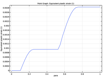
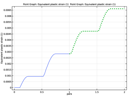
In the Settings window for Point Graph, click Replace Expression in the upper-right corner of the y-Axis Data section. From the menu, choose Component 1 (comp1)>Solid Mechanics>Strain>solid.epe - Equivalent plastic strain.
|
|
4
|
|
1
|
|
2
|
|
1
|
|
3
|
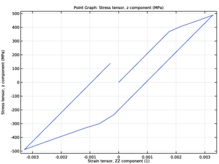
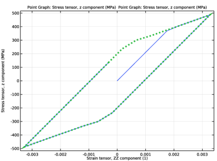
In the Settings window for Point Graph, click Replace Expression in the upper-right corner of the y-Axis Data section. From the menu, choose Component 1 (comp1)>Solid Mechanics>Stress>Stress tensor (spatial frame) - N/m²>solid.sz - Stress tensor, z component.
|
|
4
|
|
5
|
Click Replace Expression in the upper-right corner of the x-Axis Data section. From the menu, choose Component 1 (comp1)>Solid Mechanics>Strain>Strain tensor (material and geometry frames)>solid.eZZ - Strain tensor, ZZ component.
|
|
6
|
|
1
|
|
2
|
|
3
|
|
4
|
|
5
|
|
1
|
|
2
|
|
3
|
Click
|
|
5
|
Click to expand the Values of Dependent Variables section. Find the Initial values of variables solved for subsection. From the Settings list, choose User controlled.
|
|
6
|
|
7
|
|
8
|
|
9
|
|
10
|
|
11
|
|
1
|
In the Model Builder window, under Results>Plastic Strain right-click Point Graph 1 and choose Duplicate.
|
|
2
|
|
3
|
|
4
|
Click to expand the Coloring and Style section. Find the Line style subsection. From the Line list, choose Dotted.
|
|
5
|
|
6
|
|
1
|
In the Model Builder window, under Results>Stress vs. Strain right-click Point Graph 1 and choose Duplicate.
|
|
2
|
|
3
|
|
4
|
Locate the Coloring and Style section. Find the Line style subsection. From the Line list, choose Dotted.
|
|
5
|
|
6
|
|
1
|
|
2
|
|
3
|
|
4
|
Find the Physics interfaces in study subsection. In the table, clear the Solve check boxes for Study 1 (First Load Cycle) and Study 2 (Steady State Load Cycle).
|
|
5
|
|
6
|
|
1
|
|
2
|
|
3
|
|
4
|
|
5
|
Locate the Evaluation Settings section. Find the Critical plane settings subsection. In the Q text field, type 16.
|
|
1
|
In the Model Builder window, under Component 1 (comp1) right-click Materials and choose Blank Material.
|
|
2
|
|
3
|
|
4
|
|
5
|
|
1
|
|
2
|
|
3
|
Find the Physics interfaces in study subsection. In the table, clear the Solve check box for Solid Mechanics (solid).
|
|
4
|
Find the Studies subsection. In the Select Study tree, select Preset Studies for Selected Physics Interfaces>Fatigue.
|
|
5
|
|
6
|
|
1
|
|
2
|
Find the Values of variables not solved for subsection. From the Settings list, choose User controlled.
|
|
3
|
|
4
|
|
5
|
|
6
|
|
7
|
|
1
|
|
2
|
|
3
|
|
1
|
|
2
|
|
3
|
|
4
|