PDF

Notch Approximation to Low-Cycle Fatigue Analysis of Cylinder with a Hole
Introduction
A load carrying component of a structure is subjected to multiaxial cyclic loading during which a localized yielding of the material occurs. In this model you perform a low cycle fatigue analysis of the part based on the Smith-Watson-Topper (SWT) model. Due to localized yielding, you can use two methods to obtain the stress and strain distributions for the fatigue evaluation. The first method is an elastoplastic analysis with linear kinematic hardening, while the second is a linear elastic analysis with Neuber correction for plasticity, based on the Ramberg-Osgood model. This example explores the second method. In the model Elastoplastic Low-Cycle Fatigue Analysis of Cylinder with a Hole, the same problem is solved using the full elastoplastic approach.
Model Definition
Geometry
A cylinder contains a hole, drilled perpendicularly to its axis. The outer and inner diameters of the cylinder are 200 and 180 mm, respectively. Its height is 100 mm. The diameter of the hole is 20 mm. The cylinder is loaded by an axial force that varies in time.
As the structure and loading contain several symmetries, you can model only 1/8 of the cylinder, a shown in Figure 1.
Figure 1: Model geometry with constrained and loaded faces.
Material properties
Elastic data: Isotropic with E = 210 GPa, ν = 0.3
-
σf' = 1323 MPa
-
b = -0.097
-
εf' = 0.375
-
c = -0.60
Constraints
Apply symmetry conditions on the three symmetry sections shown in Figure 1.
Load
The loaded boundary of the cylinder is subjected to a pressure varying between +200 MPa and -200 MPa.
Results and Discussion
The von Mises stress distribution at maximum load is shown in Figure 2. Notice that the yield limit(380 = MPa) is extensively exceeded, so in reality significant plastic strains can be expected.
Figure 2: von Mises stress level at the first maximum load
The computed number of cycles to fatigue is shown in Figure 3. It is slightly below 5000 cycles.
Figure 3: The distribution of expected number of cycles at the hole.
Notes About the COMSOL Implementation
When using the elastic approach to low cycle fatigue, it is only the peak loads that are important, not the load cycle as such. The model includes both the maximum and the minimum loads, since some of the criteria are sensitive to the sign of the stresses. It is also necessary to include the “zero” load case, which contains no loads.
Application Library path: Fatigue_Module/Strain_Based/cylinder_with_hole_elastic
Modeling Instructions
From the File menu, choose New.
New
In the New window, click  Model Wizard.
Model Wizard
1
In the Model Wizard window, click  3D.
2
In the Select Physics tree, select Structural Mechanics>Solid Mechanics (solid).
3
Click Add.
4
Click  Study.
5
In the Select Study tree, select General Studies>Stationary.
6
Geometry 1
1
In the Model Builder window, under Component 1 (comp1) click Geometry 1.
2
In the Settings window for Geometry, locate the Units section.
3
From the Length unit list, choose mm.
Cylinder 1 (cyl1)
1
In the Geometry toolbar, click  Cylinder.
2
In the Settings window for Cylinder, locate the Size and Shape section.
3
In the Radius text field, type 100.
4
In the Height text field, type 100.
Cylinder 2 (cyl2)
1
Right-click Cylinder 1 (cyl1) and choose Duplicate.
2
In the Settings window for Cylinder, locate the Size and Shape section.
3
In the Radius text field, type 90.
Difference 1 (dif1)
1
In the Geometry toolbar, click  Booleans and Partitions and choose Difference.
2
3
In the Settings window for Difference, locate the Difference section.
4
Find the Objects to subtract subsection. Select the  Activate Selection toggle button.
5
6
Click  Build All Objects.
Cylinder 3 (cyl3)
1
In the Geometry toolbar, click  Cylinder.
2
In the Settings window for Cylinder, locate the Size and Shape section.
3
In the Radius text field, type 10.
4
In the Height text field, type 220.
5
Locate the Position section. In the y text field, type -110.
6
In the z text field, type 50.
7
Locate the Axis section. From the Axis type list, choose y-axis.
8
Click  Build All Objects.
Difference 2 (dif2)
1
In the Geometry toolbar, click  Booleans and Partitions and choose Difference.
2
3
In the Settings window for Difference, locate the Difference section.
4
Find the Objects to subtract subsection. Select the  Activate Selection toggle button.
5
6
Click  Build All Objects.
Block 1 (blk1)
1
In the Geometry toolbar, click  Block.
2
In the Settings window for Block, locate the Size and Shape section.
3
In the Width text field, type 100.
4
In the Depth text field, type 100.
5
In the Height text field, type 50.
6
Click  Build All Objects.
Intersection 1 (int1)
1
In the Geometry toolbar, click  Booleans and Partitions and choose Intersection.
2
Click in the Graphics window and then press Ctrl+A to select both objects.
3
In the Settings window for Intersection, click  Build All Objects.
4
Click the  Zoom Extents button in the Graphics toolbar.
Solid Mechanics (solid)
Symmetry 1
1
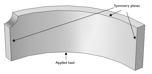
In the Model Builder window, under Component 1 (comp1) right-click Solid Mechanics (solid) and choose More Constraints>Symmetry.
2
Boundary Load 1
1
In the Physics toolbar, click  Boundaries and choose Boundary Load.
2
3
In the Settings window for Boundary Load, locate the Force section.
4
Specify the FA vector as
5
In the Physics toolbar, click  Load Group and choose New Load Group.
Materials
Material 1 (mat1)
1
In the Model Builder window, under Component 1 (comp1) right-click Materials and choose Blank Material.
2
In the Settings window for Material, locate the Material Contents section.
3
Mesh 1
Free Tetrahedral 1
In the Mesh toolbar, click  Free Tetrahedral.
Size 1
1
Right-click Free Tetrahedral 1 and choose Size.
2
In the Settings window for Size, locate the Geometric Entity Selection section.
3
From the Geometric entity level list, choose Boundary.
4
5
Locate the Element Size section. Click the Custom button.
6
Locate the Element Size Parameters section. Select the Maximum element size check box.
7
8
Click  Build All.
Study 1
Step 1: Stationary
1
In the Model Builder window, under Study 1 click Step 1: Stationary.
2
In the Settings window for Stationary, click to expand the Study Extensions section.
3
Select the Define load cases check box.
In an analysis of this type you should always supply the maximum and the minimum load, and also a zero solution.
4
Click Add three times.
5
6
In the Home toolbar, click  Compute.
Results
Surface 1
1
In the Model Builder window, expand the Results>Stress (solid) node, then click Surface 1.
2
In the Settings window for Surface, locate the Expression section.
3
From the Unit list, choose MPa.
4
In the Stress (solid) toolbar, click  Plot.
Add Physics
1
In the Home toolbar, click  Add Physics to open the Add Physics window.
2
Go to the Add Physics window.
3
In the tree, select Structural Mechanics>Fatigue (ftg).
4
Find the Physics interfaces in study subsection. In the table, clear the Solve check box for Study 1.
5
Click Add to Component 1 in the window toolbar.
6
In the Home toolbar, click  Add Physics to close the Add Physics window.
Fatigue (ftg)
Strain-Based 1
1
Right-click Component 1 (comp1)>Fatigue (ftg) and choose the boundary evaluation Strain-Based.
2
As the elastic approach to strain based fatigue is based on a notch assumption, it only makes sense to select boundaries at the hole.
3
In the Settings window for Strain-Based, locate the Fatigue Model Selection section.
4
From the Solution type list, choose Elastic solution with notch assumption.
5
Locate the Solution Field section. From the Physics interface list, choose Solid Mechanics (solid).
Materials
Material 2 (mat2)
1
In the Model Builder window, under Component 1 (comp1) right-click Materials and choose Blank Material.
2
In the Settings window for Material, locate the Geometric Entity Selection section.
3
From the Geometric entity level list, choose Boundary.
4
From the Selection list, choose All boundaries.
5
Locate the Material Contents section. In the table, enter the following settings:
Add Study
1
In the Home toolbar, click  Add Study to open the Add Study window.
2
Go to the Add Study window.
3
Find the Physics interfaces in study subsection. In the table, clear the Solve check box for Solid Mechanics (solid).
4
Find the Studies subsection. In the Select Study tree, select Preset Studies for Selected Physics Interfaces>Fatigue.
5
Click Add Study in the window toolbar.
6
In the Home toolbar, click  Add Study to close the Add Study window.
Study 2
Step 1: Fatigue
1
In the Settings window for Fatigue, locate the Values of Dependent Variables section.
2
Find the Values of variables not solved for subsection. From the Settings list, choose User controlled.
3
From the Method list, choose Solution.
4
From the Study list, choose Study 1, Stationary.
5
In the Home toolbar, click  Compute.
Results
Cycles to Failure (ftg)
The plot of cycles to failure shown in Figure 3 is created automatically.