PDF

Corrosion Protection of an Oil Platform Using Sacrificial Anodes
Introduction
Steel structures immersed in seawater can be protected from corrosion through cathodic protection. This protection can be achieved by an impressed external current or by using sacrificial anodes. The use of sacrificial anodes is often preferred due to its simplicity.
The principle for cathodic protection using sacrificial anodes is quite simple: the steel structure is electronically connected to a less noble metal, for example aluminum, which causes the sacrificial anode to be anodically polarized and the steel structure to be cathodically polarized when the electrodes are immersed in seawater. The anodes are dissolved through anodic dissolution of the metal while oxygen reduction takes place at the surface of the steel structure. The supply of oxygen is what often limits the current density for oxygen reduction, which means that a limiting current of an almost constant value over a few hundreds of millivolts in potential is obtained at the surface of the steel structure.
Figure 1: Polarization behavior of the sacrificial anodes (blue) and steel surface (red).
Figure 1 above shows the schematic polarization of the sacrificial anodes and of the oxygen reduction reaction at the surface of the steel structure. The red curve represents the polarization of the steel surface while the blue curve is the polarization of the sacrificial anode. On the left, the currents at the steel structure (red) and at the sacrificial anodes (blue) are plotted as functions of the electric potential measured relative to a common reference. The plot to the right shows the electric potential as a function of the logarithm of the absolute value of the current. As shown in the left graphs, oxygen reduction is achieved at the steel surface along the range of the cathodic limiting current represented by the flat horizontal part of the red curve. In the right plot, the vertical part of the red curve represents oxygen reduction. The system operates at the point where the cathodic current (red) is equal in size (but opposite in sign) as the anodic current.
The shape of the blue curve changes depending on the number and design of the anodes in the system, and the designer of the system needs to ensure that the different parts of the steel structure are well within the corrosion protected range of potentials (the “flat” part of the red cathodic curve); otherwise the structure is not fully protected and may start to corrode. The width of the oxygen reduction part of the curve is a few hundred millivolts. In addition, the anodes have to be able to deliver the required potential to keep the given current.
The first step in the design of a cathodic protection system is therefore to investigate the potential of the steel structure assuming a constant cathodic current (oxygen reduction). The potential has to be well within the required range where oxygen reduction protects the structure and also avoiding hydrogen evolution, which may eventually cause hydrogen embrittlement.
This example is based on a Recommended Practice for Cathodic Protection Design by DNV (Ref. 1).
Model Definition
Figure 2 and Figure 3 show the model geometry. The sacrificial anodes are placed relatively close to the oil platform. The radius of the inner cylinder is chosen so that the main part of the charge transport occurs within this cylinder. The outer cylinder is modeled as an infinite Element Domain, which rescales the equations to represent an approximately thousand times larger cylinder.
Figure 2: Model geometry.
Figure 3: Close-up view of the cylindrical sacrificial anodes and the oil platform structure.
In seawater, the composition is assumed to vary to a very small extent and diffusion of the ions that carry the current is negligible compared to the contribution from migration of these ions in the electric field. This assumption, together with the boundary conditions, allows using a primary current density distribution analysis on the system where only the influence of ohmic effects in the given geometry are taken into account.
At the sacrificial anode surfaces, a constant potential is set assuming a relatively fast kinetics. This assumption implies that a very small change in surface overpotential leads to a very large change in current density and it is therefore reasonable to set a constant potential. Grounding the electronic phase potential (setting it to zero), the boundary condition for the electrolyte phase potential is:
(1)
The value for the equilibrium potential of the aluminum anodes is -1.05 V vs Ag/AgCl in this model.
At the steel surface, it is assumed that oxygen reduction takes place at a limiting current density, limited to the rate of transport of dissolved oxygen to the surface, and that the surface is sufficiently protected so that metal dissolution currents can be neglected. This yields a constant normal current density boundary condition at the steel surfaces of the structure. The boundary condition for the steel surface is:
(2)
The value for the limiting current is 0.1 A/m2 in this model.
All other boundaries are insulated.
The model can be easily extended to secondary current density distribution analysis in order to add the kinetics of the electrode reactions in a second stage, see for instance the Anode Film Resistance Effect on Cathodic Corrosion Protection example. A tertiary current density distribution analysis that also accounts for the transport of charged species is also possible in the Corrosion Module, although this would require the use of different physics interfaces.
Results and Discussion
Figure 4 shows a slice plot of the potential in the electrolyte, . The potential close to the steel structure surface varies several hundreds of millivolts, depending on position. The further the distance from an anode – the lower the potential, an expected result since the current in the electrolyte flows from the anodes to the steel cathode.
Figure 4: Slice plot of the electrolyte potential.
One can relate the electrolyte potential, , to the electrode potential, shown in Figure 1, by considering a reference electrode placed in the electrolyte in close vicinity to the steel surface. The electric potential of a reference electrode, , is
(3)
The electric potential of the steel surface, , is constant due to the high conductivity of the metal, and the potential of the steel surface versus the reference electrode becomes
(4)
In this model we chose the metal potential as ground, and assuming a Ag/AgCl reference we get:
(5)
Figure 5 shows the potential of the steel surface according to Equation 5. The parts of the steel surface with the highest (most anodic) values in this plot are the least protected.
Figure 5: Steel platform potential vs a Ag/AgCl reference.
Figure 6 shows a close-up of one of the structure legs. The inside bottom part of the leg is the part most susceptible to corrosion.
Figure 6: Potential on one of the legs of the platform structure.
Finally, Figure 7 shows the current densities on the anodes, which are of interest because their magnitudes are directly proportional to the consumption rate of the anode metal. The highest current density for the anodes is about four times the lowest current density.
Figure 7: Current densities on the anodes.
Reference
1. Det Norske Veritas, Recommended Practice Cathodic Protection Design, NDV-RP-B401, October 2010.
Application Library path: Corrosion_Module/Cathodic_Protection/oil_platform
Modeling Instructions
From the File menu, choose New.
New
In the New window, click  Model Wizard.
Model Wizard
1
In the Model Wizard window, click  3D.
2
In the Select Physics tree, select Electrochemistry>Primary and Secondary Current Distribution>Primary Current Distribution (cd).
3
Click Add.
4
Click  Study.
5
In the Select Study tree, select General Studies>Stationary.
6
Global Definitions
Add some parameters for use in the model.
Parameters 1
1
In the Model Builder window, under Global Definitions click Parameters 1.
2
In the Settings window for Parameters, locate the Parameters section.
3
Geometry 1
Import the geometry of the oil platform from a geometry file.
Import 1 (imp1)
1
In the Home toolbar, click  Import.
2
In the Settings window for Import, locate the Import section.
3
Click Browse.
4
5
Click Import.
6
Locate the Selections of Resulting Entities section. Select the Resulting objects selection check box.
7
From the Show in physics list, choose Boundary selection.
8
Select the Individual object selections check box.
9
From the Show in physics list, choose Boundary selection.
This generates selections of the imported geometry, which you will use later on when setting up the physics on the boundaries (the anodes and the steel structure).
10
Click  Build Selected.
Cylinder 1 (cyl1)
Add a surrounding cylinder around the platform.
1
In the Geometry toolbar, click  Cylinder.
2
In the Settings window for Cylinder, locate the Size and Shape section.
3
In the Radius text field, type 40.
4
In the Height text field, type 92.
Add a second cylinder with a larger radius, this cylinder will be used to define an Infinite Element Domain.
Cylinder 2 (cyl2)
1
Right-click Cylinder 1 (cyl1) and choose Duplicate.
2
In the Settings window for Cylinder, locate the Size and Shape section.
3
In the Radius text field, type 60.
4
Click the  Wireframe Rendering button in the Graphics toolbar.
5
Click the  Zoom Extents button in the Graphics toolbar.
Difference 1 (dif1)
Create the final geometry as the difference between the cylinders and the imported oil platform structure.
1
In the Geometry toolbar, click  Booleans and Partitions and choose Difference.
2
Select the objects cyl1 and cyl2 only.
3
In the Settings window for Difference, locate the Difference section.
4
Find the Objects to subtract subsection. Select the  Activate Selection toggle button.
5
Use the Select Box toolbar button to select the imported platform geometry.
6
Click  Build Selected.
7
Click the  Zoom Extents button in the Graphics toolbar.
The finalized geometry should now look like that in the figure below.
Definitions
Now set the outer cylinder to be an Infinite Element Domain, this will scale the equations of the outer cylinder to have an approximately 1000 times larger radius.
Infinite Element Domain 1 (ie1)
1
In the Model Builder window, expand the Component 1 (comp1)>Definitions node.
2
Right-click Definitions and choose Infinite Element Domain.
3
4
In the Settings window for Infinite Element Domain, locate the Geometry section.
5
From the Type list, choose Cylindrical.
Anodes
Create a selection for the anodes by using a difference between selections that were created (by enabling Create selections) by the geometry node.
1
In the Definitions toolbar, click  Difference.
2
In the Settings window for Difference, locate the Geometric Entity Level section.
3
From the Level list, choose Boundary.
4
Locate the Input Entities section. Under Selections to add, click  Add.
5
In the Add dialog box, select Import 1 in the Selections to add list.
6
7
In the Settings window for Difference, locate the Input Entities section.
8
Under Selections to subtract, click  Add.
9
In the Add dialog box, select Object 41 (Import 1) in the Selections to subtract list.
10
11
Right-click Difference 1 and choose Rename.
12
In the Rename Difference dialog box, type Anodes in the New label text field.
13
Materials
Set the sea water conductivity in the Materials node.
Material 1 (mat1)
1
In the Model Builder window, under Component 1 (comp1) right-click Materials and choose Blank Material.
2
In the Settings window for Material, click to expand the Material Properties section.
3
Click to collapse the Material Properties section. Locate the Material Contents section. In the table, enter the following settings:
Primary Current Distribution (cd)
Now add boundary conditions for the anodes and the steel structure.
Electrode Surface - Anodes
1
In the Model Builder window, under Component 1 (comp1) right-click Primary Current Distribution (cd) and choose Electrode Surface.
2
In the Settings window for Electrode Surface, type Electrode Surface - Anodes in the Label text field.
3
Locate the Boundary Selection section. From the Selection list, choose Anodes.
Electrode Reaction 1
1
In the Model Builder window, expand the Electrode Surface - Anodes node, then click Electrode Reaction 1.
2
In the Settings window for Electrode Reaction, locate the Equilibrium Potential section.
3
In the Eeq text field, type Eeq_Al.
Electrolyte Current Density - Steel
1
In the Physics toolbar, click  Boundaries and choose Electrolyte Current Density.
2
In the Settings window for Electrolyte Current Density, type Electrolyte Current Density - Steel in the Label text field.
3
Locate the Boundary Selection section. From the Selection list, choose Object 41 (Import 1).
4
Locate the Electrolyte Current Density section. In the in,l text field, type i_oxygen.
Mesh 1
1
In the Model Builder window, under Component 1 (comp1) click Mesh 1.
2
In the Settings window for Mesh, locate the Mesh Settings section.
3
From the Sequence type list, choose User-controlled mesh.
Size
1
In the Model Builder window, under Component 1 (comp1)>Mesh 1 click Size.
2
In the Settings window for Size, locate the Element Size section.
3
Click the Custom button.
4
Locate the Element Size Parameters section. In the Maximum element size text field, type 10.
5
In the Minimum element size text field, type 0.5.
6
In the Curvature factor text field, type 0.9.
The physics is now complete. Add mesh settings and solve the model.
7
In the Model Builder window, click Size.
8
In the Settings window for Size, locate the Element Size Parameters section.
9
In the Maximum element size text field, type 15.
Free Triangular 1
1
In the Mesh toolbar, click  Boundary and choose Free Triangular.
2
Right-click Free Triangular 1 and choose Move Up.
3
In the Settings window for Free Triangular, locate the Boundary Selection section.
4
Click  Paste Selection.
5
In the Paste Selection dialog box, type 17 19 145 147 314 316 368 370 in the Selection text field.
6
Size 1
1
Right-click Free Triangular 1 and choose Size.
2
In the Settings window for Size, locate the Element Size section.
3
Click the Custom button.
4
Locate the Element Size Parameters section. Select the Minimum element size check box.
5
6
Click  Build All.
Study 1
1
In the Model Builder window, click Study 1.
2
In the Settings window for Study, locate the Study Settings section.
3
Clear the Generate default plots check box.
4
In the Home toolbar, click  Compute.
Results
Proceed as follows to create a slice plot of the electrolyte potential:
Electrolyte potential
1
In the Home toolbar, click  Add Plot Group and choose 3D Plot Group.
2
In the Settings window for 3D Plot Group, type Electrolyte potential in the Label text field.
Slice 1
1
Right-click Electrolyte potential and choose Slice.
2
In the Settings window for Slice, locate the Plane Data section.
3
From the Plane list, choose ZX-planes.
4
In the Planes text field, type 1.
5
Click the  Zoom Extents button in the Graphics toolbar.
6
In the Electrolyte potential toolbar, click  Plot.
Compare with Figure 4.
Steel potential
Plot the potential along the steel boundaries by first adding a selection for these boundaries.
1
In the Home toolbar, click  Add Plot Group and choose 3D Plot Group.
2
In the Settings window for 3D Plot Group, type Steel potential in the Label text field.
3
Click to expand the Title section. From the Title type list, choose Manual.
4
In the Title text area, type Steel potential vs. Ag/AgCl (V).
5
Locate the Plot Settings section. Clear the Plot dataset edges check box.
Surface 1
1
Right-click Steel potential and choose Surface.
2
In the Settings window for Surface, locate the Expression section.
3
In the Expression text field, type -phil.
Selection 1
1
Right-click Surface 1 and choose Selection.
2
In the Settings window for Selection, locate the Selection section.
3
From the Selection list, choose Object 41 (Import 1).
4
Click the  Zoom Extents button in the Graphics toolbar.
5
In the Steel potential toolbar, click  Plot.
The plot should look like that in Figure 5.
Steel potential
Proceed in a similar way to plot the potential along a close-up of one of the platform legs.
Steel potential 1
1
In the Model Builder window, right-click Steel potential and choose Duplicate.
2
Expand the Steel potential 1 node.
Selection 1
1
In the Model Builder window, expand the Results>Steel potential 1>Surface 1 node, then click Selection 1.
2
In the Settings window for Selection, locate the Selection section.
3
From the Selection list, choose Manual.
4
Click  Clear Selection.
5
Click  Paste Selection.
6
In the Paste Selection dialog box, type 212-214, 218-220, 223-224 in the Selection text field.
7
Steel potential, close-up
1
In the Model Builder window, right-click Steel potential 1 and choose Rename.
2
In the Rename 3D Plot Group dialog box, type Steel potential, close-up in the New label text field.
3
4
Click the  Zoom Extents button in the Graphics toolbar.
5
In the Steel potential, close-up toolbar, click  Plot.
Compare the resulting plot with that in Figure 6.
Anode current densities
Finally, proceed in the following way to plot the current density on the anodes.
1
Right-click Steel potential, close-up and choose Duplicate.
2
In the Model Builder window, click Steel potential, close-up 1.
3
In the Settings window for 3D Plot Group, type Anode current densities in the Label text field.
4
Locate the Title section. In the Title text area, type Anode current densities (A/m<sup>2</sup>).
Surface 1
1
In the Model Builder window, click Surface 1.
2
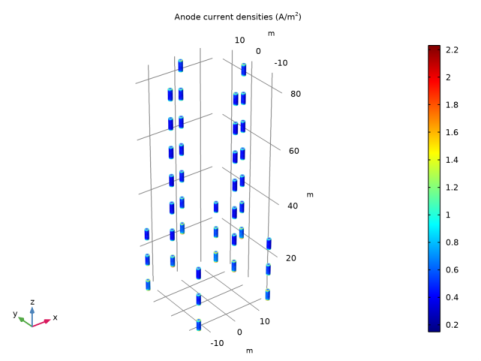
In the Settings window for Surface, click Replace Expression in the upper-right corner of the Expression section. From the menu, choose Component 1 (comp1)>Primary Current Distribution>cd.nIl - Normal electrolyte current density - A/m².
3
Locate the Expression section. In the Expression text field, type abs(cd.nIl).
Selection 1
1
In the Model Builder window, expand the Surface 1 node, then click Selection 1.
2
In the Settings window for Selection, locate the Selection section.
3
From the Selection list, choose Anodes.
4
Select the  Activate Selection toggle button.
5
In the Anode current densities toolbar, click  Plot.
6
Click the  Zoom Extents button in the Graphics toolbar.
Compare with Figure 7.