
|
|
|
|
1
|
|
2
|
In the Select Physics tree, select Electrochemistry>Primary and Secondary Current Distribution>Current Distribution, Boundary Elements (cdbem).
|
|
3
|
Click Add.
|
|
4
|
Click
|
|
5
|
|
6
|
Click
|
|
1
|
|
2
|
|
3
|
Click Browse.
|
|
4
|
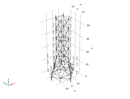
Browse to the model’s Application Libraries folder and double-click the file oil_platform_wireframe.mphbin.
|
|
5
|
Click Import.
|
|
1
|
|
2
|
|
3
|
|
4
|
|
5
|
In the Paste Selection dialog box, type 10-22, 123-129, 154-160, 225-237 in the Selection text field.
|
|
6
|
Click OK.
|
|
7
|
|
1
|
|
2
|
|
3
|
|
4
|
|
5
|
In the Paste Selection dialog box, type 1-9,23-122, 130-153, 161-224, 238-240 in the Selection text field.
|
|
6
|
Click OK.
|
|
7
|
|
1
|
|
2
|
|
3
|
|
4
|
|
5
|
In the Paste Selection dialog box, type 1, 4, 7, 117, 119, 121, 161, 163, 165, 238-240 in the Selection text field.
|
|
6
|
Click OK.
|
|
7
|
|
1
|
|
2
|
|
3
|
|
4
|
|
5
|
In the Paste Selection dialog box, type 2-3, 26, 29, 42-45, 50, 57, 64, 71, 90-93, 96, 100, 104, 108, 111, 114, 118, 162, 167, 170, 173-176, 179, 183, 187, 191, 204-211, 221, 223 in the Selection text field.
|
|
6
|
Click OK.
|
|
7
|
|
1
|
|
2
|
|
3
|
|
4
|
|
5
|
In the Paste Selection dialog box, type 5-6, 32, 35, 46, 48, 53, 56, 59, 62, 67, 70, 73, 75-76, 83, 94, 99, 102, 107, 110, 120, 130, 136, 143, 149, 164, 177, 182, 185, 190, 193-194, 199, 217, 219 in the Selection text field.
|
|
6
|
Click OK.
|
|
7
|
|
1
|
|
2
|
|
3
|
|
4
|
|
5
|
|
6
|
Click OK.
|
|
7
|
|
8
|
|
9
|
|
10
|
Click OK.
|
|
11
|
|
1
|
In the Model Builder window, under Component 1 (comp1) click Current Distribution, Boundary Elements (cdbem).
|
|
2
|
In the Settings window for Current Distribution, Boundary Elements, click to expand the Symmetry section.
|
|
3
|
|
1
|
In the Model Builder window, under Component 1 (comp1)>Current Distribution, Boundary Elements (cdbem) click Electrolyte 1.
|
|
2
|
|
3
|
|
1
|
|
2
|
|
3
|
|
4
|
|
5
|
|
1
|
|
2
|
|
3
|
|
4
|
|
5
|
|
1
|
|
2
|
|
3
|
|
4
|
|
5
|
|
1
|
|
2
|
|
3
|
|
4
|
|
5
|
|
1
|
|
2
|
|
3
|
|
4
|
|
5
|
|
1
|
|
2
|
|
3
|
|
4
|
|
1
|
|
2
|
|
1
|
|
2
|
|
3
|
|
4
|
|
5
|
|
6
|
|
1
|
|
2
|
In the Settings window for 3D Plot Group, type Normal Electrolyte Current Density in the Label text field.
|
|
1
|
|
2
|
|
3
|
|
4
|
|
1
|
|
2
|
|
1
|
|
2
|
|
1
|
|
2
|
|
1
|
|
2
|
Select the object imp1 only.
|
|
3
|
|
4
|
|
5
|
|
6
|
|
7
|
|
8
|
|
1
|
|
1
|
|
2
|
|
1
|
|
2
|
|
3
|
|
4
|
|
1
|
|
2
|
|
3
|
|
1
|
|
2
|
|
3
|
|
4
|
|
5
|