Localized Corrosion Using the Level Set Method

This example models the galvanic corrosion between the two constituent phases of a metallic alloy. Since the two phases have different equilibrium potentials corrosion occurs when the alloy is exposed to an electrolyte solution. While similar to the Localized Corrosion example, the present model considers a different cross-sectional microstructure that could potentially lead to topological changes. Since the deformed geometry formulation used in the Localized Corrosion example cannot handle topological changes, the Level Set method is used in the present model to capture dissolution of a constituent phase.

This model example is based on a paper by Deshpande (Ref. 1).

Model Definition

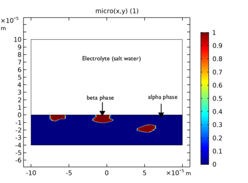
The model geometry considered in this example is shown in Figure 1, along with a representative cross-sectional microstructure, which consists of the alpha and beta phases exposed to the electrolyte solution.

Figure 1: Model geometry along with cross-sectional microstructure comprising of the alpha and beta phases and exposed to the electrolyte solution.

The cross-sectional microstructure shown in Figure 1 is represented in terms of an interpolation function called “micro” which has a value of 0 and 1 for the alpha and beta phases, respectively. The metal alloy geometry has a width of 200 μm and a depth of 40 μm. The maximum depth of the beta phase is 10 μm.

Electrolyte charge transport

Use the Secondary Current Distribution interface to solve for the electrolyte potential,

, over the electrolyte domain according to Ohm’s law:

where il (SI unit: A/m2) is the electrolyte current density vector.

The electrolyte conductivity, σl (SI unit: S/m), is defined for the electrolyte and electrode domains separately in terms of level set variable,

, according to

where σel is the electrolyte conductivity in the electrolyte domain and is considered to be equal to 2.5 S/m and σed is the electrolyte conductivity in the electrode domain and is considered to be equal to 0.1 S/m. While the electrolyte conductivity in electrolyte domain describes the actual chemistry of the problem, the electrolyte conductivity in the electrode domain is defined only to aid numerical convergence.

Use the default Insulation condition for all exterior boundaries:

where n is the normal vector, pointing out of the domain.

Use an Electrolyte Current Source domain node to define the electrode kinetics at the corroding boundary:

where iloc (SI unit: A/m2) is the local electrode reaction current density and δ (SI unit: 1/m) is the level set delta function.

Use a user-defined electrode kinetics expression to model the electrode reaction at the alpha and beta phases on the electrode surface.

Set the local current density for the alpha phase at the electrode surface to

The 1-micro(x,y) factor ensures that the local current density is applied only at the alpha phase on the electrode surface.

The interpolation function micro(x,y) ensures that the local current density is applied only at the beta phase on the electrode surface.

A relationship between the local current density and the electrolyte potential,

, is incorporated in the model using a piecewise cubic interpolation function for the experimental polarization data. The same polarization data as used in the Localized Corrosion example is used here for the alpha and beta phases.

Set the local current density for the alpha and beta phases at the electrode surface according to

Corrosion interface tracking

Use the Level Set interface to keep track of dissolution of the alpha phase. The Level Set interface automatically sets up the equations for the movement of the interface between the electrolyte and electrode domains. The interface is represented by the 0.5 contour of the level set variable

. The level set variable varies from 1 in the electrode domain to 0 in the electrolyte domain. The transport of the level set variable is given by:

The ε parameter determines the thickness of the interface and is defined as ε = hmax/4, where hmax is the maximum mesh element size in the domain. The γ parameter determines the amount of reinitialization. A suitable value for γ is the maximum velocity magnitude occurring in the model.

The level set delta function is approximated by:

In this model formulation, it is assumed that the anodic dissolution reaction takes place at the alpha phase surface, and that the cathodic hydrogen evolution reaction (which is not associated with any loss of material) takes place at the beta phase surface. Hence, the alpha phase surface will move (dissolve) whereas the beta phase surface remains intact. This is achieved in the model by setting the alpha phase dissolution velocity in normal direction according to

where MMg is the mean molar mass (23.98 g/mol) and ρMg is the density (1770 kg/m3) of the magnesium alloy.

Use the Inlet boundary node for the exterior boundaries of the electrolyte domain and set the level set variable to 0 at those boundaries.

Use the Outlet boundary node for the exterior boundaries of the electrode domain.

To set the initial interface position, use the Initial Interface boundary node for the interior boundary between the electrolyte and electrode domains.

Results and Discussion

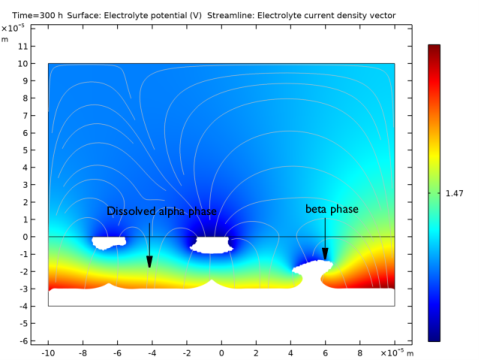
Figure 2 shows a surface plot of the electrolyte potential at time t = 300 h. It can be seen that the alpha phase, being electrochemically more active, is dissolving from the electrode surface whereas the beta phase, being relatively nobler, remains intact. With the preferential dissolution of the alpha phase, the underlying beta phase gets exposed to the electrolyte solution, resulting in an increase in the surface beta phase fraction at the electrode surface. It can be seen in Figure 2 that the alpha phase in the electrode domain, as shown in Figure 1, is dissolved in the electrolyte solution. The dissolved alpha phase and intact beta phase are highlighted in Figure 2 at time t = 300 h.

Figure 2: A surface plot of the electrolyte potential at time t = 300 h where the dissolved alpha phase and intact beta phase are highlighted.

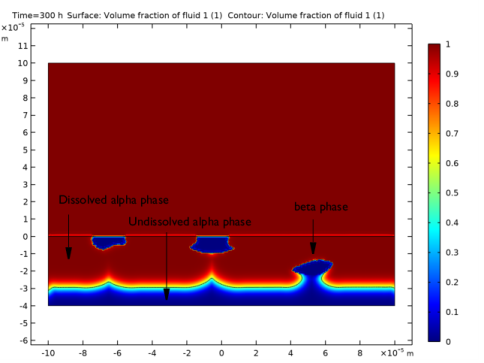
Figure 3 shows a surface plot of the volume fraction of fluid 1 at time t = 300 h. The volume fraction of value 1 represents the electrolyte domain and 0 represents the electrode domain. The dissolved alpha phase, undissolved alpha phase and intact beta phase regions of the electrode domain are highlighted in Figure 3 at time t = 300 h. Since the Level Set method can handle topological changes, the computations are continued even after the beta phase falls off the electrode surface.