Localized Corrosion

A metallic alloy with two constituent phases of different equilibrium potentials is susceptible to corrosion when it is exposed to an electrolyte solution. The constituent phase with a lower potential acts as an anode and preferentially corrodes whereas the other phase with a positive potential acts as a cathode. In order to capture the preferential dissolution of the anode phase, an explicit tracking of the dissolving interface is required which makes it a moving boundary problem.

In this model formulation, the electrode kinetics at both the anode and cathode phases are implemented in a unique way in terms of the level set function. Similarly, movement of the anode surface is implemented using the level set function and the in-built moving mesh formulation.

This model example simulates the cross-sectional microstructure evolution during a corrosion event and is based on a paper by Deshpande (Ref. 1).

Model Definition

The model geometry considered in this example is shown in Figure 1 along with a representative cross-sectional microstructure, which consists of the alpha and beta phases exposed to the electrolyte solution. The cross-sectional microstructure shown in Figure 1 is represented in terms of the level set function using an interpolation function called “micro”. It has width of 200 μm and depth of 25 μm and the maximum depth of the alpha phase is 10 μm. The alpha and beta phases at the electrode boundary are identified when the interpolated level set function, micro, has a value of 0 and 1, respectively.

Use the Secondary Current Distribution interface to solve for the electrolyte potential, φl(V), over the electrolyte domain according to:

where il (SI unit: A/m2) is the electrolyte current density vector and σl (SI unit: S/m) is the electrolyte conductivity which is assumed to be a constant of 2.5 S/m.

Use the default Insulation condition for all boundaries except the electrode surface:

where n is the normal vector, pointing out of the domain.

Figure 1: Model geometry along with cross-sectional microstructure comprising the alpha and beta phases and exposed to the electrolyte solution.

Use an Electrode Surface boundary node, with an added Dissolving-Depositing Species, at the electrode surface. This will set the boundary condition for the electrolyte potential to

where iloc,m (SI unit: A/m2) is the local individual electrode reaction current density.

The dissolution at the electrode surface with a velocity in the normal direction is evaluated according to

where Mi is the molar mass (23.98 g/mol) and ρi is the density (1770 kg/m3) of the corroding species i.

Rdep,i,m is evaluated using the following equation:

where

is the stoichiometric coefficient and nmis the number of electrons participating in the electrode reaction.

Use a User Defined electrode kinetics expression type to model the electrode reaction at the alpha phase on the electrode surface.

Set the local current density for the alpha phase at the electrode surface to

(1)

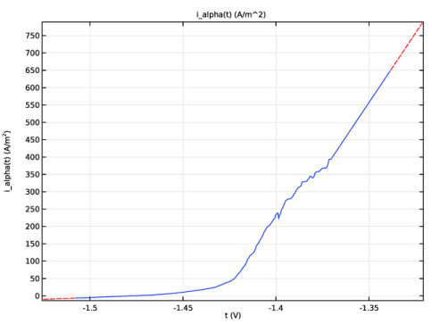
A relationship between the local current density and the electrolyte potential for the alpha phase at the electrode surface is incorporated in the model using a piecewise cubic interpolation function for the experimental polarization data as shown in Figure 2.

Figure 2: Anodic polarization data for the alpha phase.

It should be noted that the expression, 1-micro(x,y), ensures that the local current density is applied only at the alpha phase on the electrode surface.

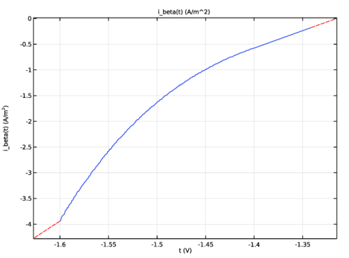
A relationship between the local current density and the electrolyte potential for the beta phase at the electrode surface is incorporated in the model using a piecewise cubic interpolation function for the experimental polarization data as shown in Figure 3. The level set function micro(x,y) ensures that the local current density is applied only at the beta phase on the electrode surface.

Figure 3: Cathodic polarization data for the beta phase.

In this model formulation, it is assumed that the anodic dissolution reaction takes place at the alpha phase surface and the cathodic hydrogen evolution reaction, where there is no material loss, takes place at the beta phase surface. Hence, the alpha phase surface is considered to be moving (dissolving) whereas the beta phase surface is considered to remain intact. This is achieved in the model by setting the value of stoichiometric coefficient to 1 and 0 for the alpha phase and beta phase electrode reactions, respectively.

The mesh used in the model is shown in Figure 4.

Figure 4: The mesh used in the model.

Results and Discussion

Figure 5 shows a surface plot of the electrolyte potential at time t = 59 h. It can be seen that the alpha phase, being electrochemically more active, is dissolving from the electrode surface whereas the beta phase, being relatively nobler, remains intact. With the preferential dissolution of the alpha phase, the underneath beta phase gets exposed to the electrolyte solution resulting in an increase in the surface beta phase fraction at the electrode surface. The computations are stopped when the surface beta phase fraction reaches a value of 0.95 which happens at time t = 59 h in this case. It can be seen in Figure 5 that most of the alpha phase shown in Figure 1 is dissolved in the electrolyte solution at time t = 59 h.

Figure 5: A surface plot of the electrolyte potential at time t = 59 h where the dissolved alpha phase and intact beta phase are highlighted.

The surface beta phase fraction at the electrode surface is evaluated using the following equation:

It can be seen in Figure 6 that the surface beta phase fraction is around 0.2 at an initial stage and it increases with time due to preferential dissolution of the alpha phase from the electrode surface exposing the underneath beta phase. The change in surface beta phase fraction with time is considerably gradual until time t = 40 h; however, it becomes more rapid for a higher value of surface beta phase fraction.

Figure 6: The change in the surface beta phase fraction with time.

The average anode current density at the electrode surface is evaluated using the following equation:

where ialpha defined in Equation 1 is used.

Figure 7 shows the change in the average anode current density with time where it is found to be gradual for the lower surface beta phase fraction, similar to the change in surface beta phase fraction. The average anode current density increases very rapidly for the higher surface beta phase fraction which is attributed to a higher cathode to anode area ratio at the electrode surface.