Two-Phase Flow Modeling of a Dense Suspension

Liquid-solid mixtures (suspensions) are important in a variety of industrial fields, such as oil and gas refinement, paper manufacturing, food processing, slurry transport, and wastewater treatment. Several different modeling approaches have been developed, ranging from discrete, particle-based methods to macroscopic, semi-empirical two-phase descriptions. Particle-based methods are suitable when there is a limited number of solid particles. When, on the other hand, there are many particles, it is better to use a macroscopic, or averaged, model that tracks the volume fractions of the phases.

The following example illustrates how you can set up a macroscopic two-phase flow model in COMSOL Multiphysics using the Phase Transport Mixture Model, Laminar Flow multiphysics interface. The model is based on the “diffusive flux” model described in Ref. 1, Ref. 2, and Ref. 3, suitable for liquid-solid mixtures with high concentrations of solid particles. It accounts for not only buoyancy effects but also shear-induced migration; that is, the tendency of particles to migrate toward regions of lower shear rates.

The model simulates the flow of a dense suspension consisting of light, solid particles in a liquid placed between two concentric cylinders. The inner cylinder rotates while the outer one is fixed.

Model Definition

A suspension is a mixture of solid particles and a liquid. The dynamics of a suspension can be modeled by a momentum transport equation for the mixture, a continuity equation, and a transport equation for the solid phase volume fraction. The Phase Transport Mixture Model, Laminar Flow multiphysics interface automatically sets up these equations. It uses the following equation to model the momentum transport:

where j is the mass-averaged mixture velocity (m/s), p denotes the pressure (Pa), g refers to the acceleration of gravity (m/s2), ε is the reduced density difference, and uslip gives the relative velocity between the solid and the liquid phases (m/s). Further,

is the mixture density, where ρf and ρs are the pure-phase densities (kg/m3) of liquid and solids, respectively, and where

is the solid-phase volume fraction (m3/m3).

Finally, μ represents the mixture viscosity (Ns/m2) according to the Krieger-type expression

(1)

where μf is the dynamic viscosity of the pure fluid and

is the maximum packing concentration.

The mixture model uses the following form of the continuity equation

(2)

The transport equation for the solid-phase volume fraction is

(3)

The solid-phase velocity, us, is given by us = j + ( 1 − cs ) uslip, where

is the dimensionless particle mass fraction and j is the mass-averaged mixture velocity (m/s). Assuming ρs is constant, this means that Equation 3 is equivalent to

(4)

Rao and others (Ref. 2) formulate the continuity equation and the particle transport in a slightly different way. Instead of the slip velocity, uslip, they define a particle flux, Js (kg /(m2·s)), and write the solid phase transport according to

(5)

By comparing Equation 5 with Equation 4, it is clear that they are equivalent if

In this example you use the model for the particle flux, Js, as suggested by Subia and others (Ref. 3) and Rao and others (Ref. 2), but the open and editable format of COMSOL Multiphysics makes it possible to specify the expression arbitrarily.

Following Rao and others, the particle flux is

Here, ust is the settling velocity (m/s) of a single particle surrounded by fluid and Dφ and Dη are empirically fitted parameters (m2) given by

where a is the particle radius (m).

The shear rate tensor,

(1/s), is given by

and its magnitude by

which for a 2-dimensional problem is

The settling velocity, ust, for a single spherical particle surrounded by pure fluid is given by

For several particles in a fluid, the settling velocity is lower. To account for the surrounding particles, the settling velocity for a single particle is multiplied by the hindering function, fh, defined as

where

is the average solid phase volume fraction in the suspension, μf is the dynamic viscosity of the pure fluid (Ns/m2), and μ is the mixture viscosity (Equation 1).

The following table gives the physical properties of the solid and the liquid phases:


Name	Value	Description
ρs	1180 kg/m3	Density of particles
ρf	1250 kg/m3	Density of pure fluid
a	678 μm	Particle radius
μf	0.589 Pa·s	Viscosity of pure fluid

Boundary Conditions

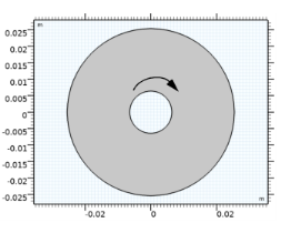
The suspension is placed in a Couette device, that is, between two concentric cylinders. The inner cylinder rotates while the outer one is fixed. The radii of the two cylinders are 0.64 cm and 2.54 cm, respectively. The inner cylinder rotates at a steady rate of 55 rpm. With the cylinder centered at (0,0), this corresponds to a velocity of

The fluid and particle motion is small along the direction of the cylinder axis. You can therefore use a 2-dimensional model. Figure 1 shows the corresponding geometry.

Figure 1: Geometry of the Couette device. The inner cylinder rotates, the outer one is fixed.

There is no particle flux through the boundaries, and the suspension velocity satisfies no slip conditions at all walls.

Initial Conditions

There are two different initial particle distributions. In the first example, the particles are evenly distributed within the device. In the second example, the particles are initially gathered at the top of the device.

Results

Case 1 — Initially Evenly Distributed Particles

A suspension with particles lighter than the fluid is placed in a concentric Couette device. Initially, the particles are evenly distributed with a constant volume fraction of 0.35. The shear rate in the device varies radially across the gap and thus it is expected that particles migrate (shear-induced migration) from regions of high shear to regions of low shear (toward the outer wall). Because the particles are lighter than the fluid, they also rise.

Figure 2: The particle concentration

at different times. The particles move to regions with lower shear rate and rise because of buoyancy.

Figure 2 shows the particle concentration

in the device at t = 0 s, t = 30 s, t = 100 s and t = 1000 s. The migration of the particles toward the outer wall is apparent. As a result of the shear induced migration and gravity, the solid phase volume fraction approaches the value for maximum packing close to the upper right outer wall. The suspension viscosity thus becomes high in this region. The results compare well with those presented in Ref. 2.

Case 2 — Particles Initially Gathered at the Top of the Device

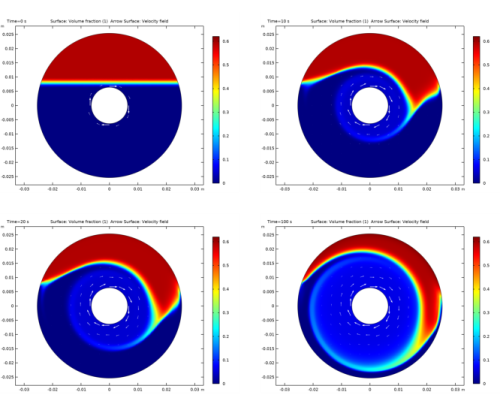
In this case the particles are initially gathered at the top of the device. The particle volume fraction is initially zero in the lower part, while it is 0.59 at the top.

Figure 3: Particle concentrations for t = 0 s, 10 s, 20 s, and100 s with particles initially at the top. Note that the same color range values are used in each of the plots.

Figure 3 shows the numerically predicted particle concentration at times 0 s, 10 s, 20 s, and 100 s. Initially, the particle motion is dominated by inertia and the effect of the shear-induced migration is not visible. At later times, shear-induced migration causes the particles to move toward the outer boundary. In this case also, the results agree well with the results in Ref. 2.

References

1. R.J. Phillips, R.C. Armstrong, R.A. Brown, A.L. Graham, and J.R. Abbot, “A Constitutive Equation for Concentrated Suspensions that Accounts for Shear-induced Particle Migration,” Phys. Fluids A, vol. 4, pp. 30–40, 1992.

2. R. Rao, L. Mondy, A. Sun, and S. Altobelli, “A Numerical and Experimental Study of Batch Sedimentation and Viscous Resuspension,” Int. J. Num. Methods in Fluids, vol. 39, pp. 465–483, 2002.

3. S.R. Subia, M.S. Ingber, L.A. Mondy, S.A. Altobelli, and A.L. Graham, “Modelling of Concentrated Suspensions Using a Continuum Constitutive Equation,” J. Fluid Mech., vol. 373, pp. 193–219, 1998.

Notes About the COMSOL Implementation

To set up the model with COMSOL Multiphysics, open the Mixture Model, Laminar Flow interface. The shear rate is discretized as an additional equation to improve accuracy because the particle flux contains derivatives of this quantity, which in turn depend on the derivatives of the velocity.

CFD_Module/Verification_Examples/dense_suspension

Modeling Instructions

From the menu, choose .

New

In the window, click

Model Wizard

In the window, click

In the tree, select .

Click .

In the tree, select .

In the table, enter the following settings:


phic
phid

In the tree, select .

Click .

In the table, enter the following settings:


gamma

Click

In the table, enter the following settings:


Dependent variable quantity	Unit
Custom unit	1/s

Click

In the table, enter the following settings:


Source term quantity	Unit
Custom unit	1/s

Click

In the tree, select .

Click

Global Definitions

Parameters 1

In the window, under click .

In the window for , locate the section.

Click

Browse to the model’s Application Libraries folder and double-click the file dense_suspension_parameters.txt.

Geometry 1

Circle 1 (c1)

In the toolbar, click

In the window for , locate the section.

In the text field, type 0.0064.

Click

Circle 2 (c2)

In the toolbar, click

In the window for , locate the section.

In the text field, type 0.0254.

Click

Difference 1 (dif1)

In the toolbar, click

and choose .

Select the object only.

In the window for , locate the section.

Find the subsection. Select the

toggle button.

Select the object only.

Click

Definitions

Variables 1

In the toolbar, click

and choose .

In the window for , locate the section.

Click

Browse to the model’s Application Libraries folder and double-click the file dense_suspension_variables.txt.

Laminar Flow (spf)

In the window, under click .

In the window for , locate the section.

Select the check box.

Pressure Point Constraint 1

In the toolbar, click

and choose .

Select Point 1 only.

Wall 2

In the toolbar, click

and choose .

Select Boundaries 3, 4, 6, and 7 only.

In the window for , click to expand the section.

From the list, choose .

Specify the utr vector as


c_vel*y	x
-c_vel*x	y

Phase Transport (phtr)

Initial Values 1

In the window, under click .

In the window for , locate the section.

In the s0,phid text field, type phi0.

General Form PDE (g)

In the window, under click .

In the window for , click to expand the section.

From the list, choose .

General Form PDE 1

In the window, under click .

In the window for , locate the section.

Specify the Γ vector as


0	x
0	y

Locate the section. In the f text field, type gamma-sqrt(0.5*(4*ux^2+2*(uy+vx)^2+4*vy^2)+eps).

Locate the section. In the da text field, type 0.

Flux/Source 1

In the toolbar, click

and choose .

In the window for , locate the section.

From the list, choose .

Multiphysics

Mixture Model 1 (mfmm1)

In the window, under click .

In the window for , locate the section.

From the list, choose . From the list, choose .

In the φmax text field, type phi_max.

Locate the section. From the ρc list, choose . In the associated text field, type rho_f.

From the μc list, choose . In the associated text field, type eta_f.

Locate the section. From the ρphid list, choose . In the associated text field, type rho_s.

Specify the uslip,phid vector as


J1/(phidrho_s(1-cd))	x
J2/(phidrho_s(1-cd))	y

Mesh 1

Free Triangular 1

In the toolbar, click

Size

In the window, click .

In the window for , locate the section.

From the list, choose .

Click the button.

Locate the section. In the text field, type 0.0012.

Click

Study 1

Step 1: Time Dependent

In the window, under click .

In the window for , locate the section.

In the text field, type 0 30 100 1000.

Solution 1 (sol1)

In the toolbar, click

In the window, expand the node.

In the window, click .

In the window for , click to expand the section.

In the toolbar, click

Results

Velocity (spf)

To visualize the volume fraction of the as a surface plot along with the mixture velocity field as an arrow surface plot, follow the steps given below.

Surface