|
|
|
|
•
|
|
•
|
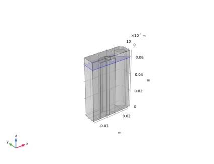
Separator (30 μm)
|
|
•
|

|
1
|
|
2
|
Browse to the model’s Application Libraries folder and double-click the file li_battery_1d_for_thermal_models.mph.
|
|
1
|
|
2
|
|
3
|
|
4
|
|
5
|
|
6
|
|
7
|
|
1
|
|
2
|
|
1
|
|
2
|
|
3
|
|
4
|
|
5
|
|
6
|
|
1
|
|
2
|
|
3
|
|
4
|
|
1
|
|
2
|
|
3
|
|
4
|
|
5
|
|
6
|
|
1
|
|
2
|
Click in the Graphics window and then press Ctrl+A to select all objects.
|
|
3
|
|
1
|
|
2
|
|
3
|
|
4
|
|
5
|
|
6
|
|
7
|
|
1
|
|
2
|
Click in the Graphics window and then press Ctrl+A to select both objects.
|
|
3
|
|
1
|
|
2
|
|
3
|
|
4
|
|
5
|
|
6
|
|
7
|
|
1
|
|
2
|
|
3
|
|
4
|
|
5
|
|
6
|
|
7
|
|
8
|
|
1
|
|
2
|
|
3
|
|
4
|
|
5
|
|
6
|
|
7
|
|
1
|
|
2
|
|
3
|
|
4
|
|
5
|
|
6
|
|
7
|
|
8
|
|
1
|
|
2
|
|
3
|
|
4
|
|
5
|
|
6
|
|
1
|
|
2
|
On the object fin, select Boundaries 6, 15, and 26 only.
|
|
3
|
|
1
|
|
2
|
|
3
|
|
4
|
Click OK.
|
|
1
|
|
2
|
|
3
|
|
4
|
Click OK.
|
|
1
|
|
2
|
|
3
|
|
4
|
Click OK.
|
|
1
|
|
2
|
|
3
|
|
4
|
Click OK.
|
|
1
|
|
2
|
|
3
|
|
4
|
Click OK.
|
|
5
|
|
6
|
|
1
|
|
2
|
|
3
|
|
4
|
Click OK.
|
|
5
|
|
6
|
|
1
|
|
2
|
|
3
|
|
4
|
Click OK.
|
|
5
|
|
6
|
|
1
|
|
2
|
|
3
|
|
4
|
Click OK.
|
|
5
|
|
6
|
|
1
|
|
2
|
|
3
|
|
1
|
In the Model Builder window, expand the Component 1 (comp1)>Definitions>Shared Properties node, then click Model Input 1.
|
|
2
|
|
3
|
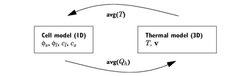
In the text field, type nojac(comp2.aveop1(comp2.T)).
|
|
1
|
|
2
|
|
3
|
|
1
|
|
2
|
Click the Component 2 node.
|
|
1
|
|
2
|
|
1
|
In the Model Builder window, expand the Domain Point Probe 1 node, then click Point Probe Expression 1 (CellVoltageProbe).
|
|
2
|
In the Settings window for Point Probe Expression, click to expand the Table and Window Settings section.
|
|
3
|
|
1
|
|
2
|
|
3
|
|
4
|
|
5
|
Click to expand the Table and Window Settings section. From the Plot window list, choose Probe Plot 1.
|
|
1
|
|
2
|
|
3
|
|
4
|
|
5
|
|
6
|
|
7
|
|
1
|
|
2
|
|
3
|
|
4
|
|
5
|
|
6
|
|
7
|
|
1
|
|
2
|
|
3
|
|
4
|
|
5
|
In the tree, select Built-in>Nylon.
|
|
6
|
|
7
|
In the tree, select Built-in>Air.
|
|
8
|
|
9
|
|
10
|
|
11
|
|
1
|
|
2
|
|
3
|
|
1
|
|
2
|
|
3
|
|
1
|
|
2
|
|
3
|
|
1
|
|
2
|
|
3
|
|
4
|
|
1
|
In the Model Builder window, under Component 2 (comp2) right-click Heat Transfer in Solids and Fluids (ht) and choose Solid.
|
|
2
|
|
3
|
|
4
|
Locate the Coordinate System Selection section. From the Coordinate system list, choose Cylindrical System 2 (sys2).
|
|
5
|
Locate the Heat Conduction, Solid section. From the k list, choose User defined. From the list, choose Diagonal.
|
|
6
|
In the k table, enter the following settings:
|
|
7
|
Locate the Thermodynamics, Solid section. From the ρ list, choose User defined. In the associated text field, type rho_batt.
|
|
8
|
|
1
|
|
2
|
|
3
|
|
4
|
|
1
|
|
2
|
|
3
|
|
1
|
In the Model Builder window, under Component 2 (comp2)>Heat Transfer in Solids and Fluids (ht) click Fluid 1.
|
|
2
|
|
3
|
|
1
|
|
2
|
|
3
|
|
4
|
|
1
|
|
2
|
|
3
|
|
1
|
|
2
|
|
3
|
|
4
|
|
1
|
|
2
|
|
3
|
|
4
|
|
1
|
|
2
|
|
3
|
|
1
|
In the Model Builder window, under Component 2 (comp2) click Heat Transfer in Solids and Fluids (ht).
|
|
2
|
|
3
|
|
1
|
In the Model Builder window, under Component 2 (comp2)>Heat Transfer in Solids and Fluids (ht) click Initial Values 1.
|
|
2
|
|
3
|
|
1
|
|
2
|
|
3
|
|
4
|
|
5
|
|
6
|
|
1
|
|
2
|
|
3
|
|
5
|
Click to expand the Sweep Method section. From the Face meshing method list, choose Triangular (generate prisms).
|
|
1
|
|
2
|
|
3
|
|
4
|
|
1
|
|
2
|
|
3
|
|
4
|
|
1
|
|
2
|
|
3
|
|
4
|
|
1
|
|
3
|
|
4
|
|
5
|
|
6
|
|
1
|
|
2
|
|
3
|
|
4
|
|
1
|
|
2
|
|
3
|
|
4
|
|
5
|
|
6
|
|
1
|
|
2
|
In the table, clear the Solve for check boxes for Lithium-Ion Battery (liion) and Heat Transfer in Solids and Fluids (ht).
|
|
3
|
|
1
|
|
2
|
In the Settings window for Current Distribution Initialization, locate the Physics and Variables Selection section.
|
|
3
|
In the table, clear the Solve for check boxes for Laminar Flow (spf) and Heat Transfer in Solids and Fluids (ht).
|
|
4
|
|
1
|
|
2
|
|
3
|
In the Output times text field, type 0 299.95 300 599.95 600 899.95 900 1199.95 1200 1499.95 1500 2100.
|
|
4
|
Locate the Physics and Variables Selection section. In the table, clear the Solve for check box for Laminar Flow (spf).
|
|
1
|
|
2
|
|
3
|
|
4
|
|
5
|
|
6
|
Click to expand the Advanced section. Locate the Time Stepping section. Find the Algebraic variable settings subsection. From the Consistent initialization list, choose Off.
|
|
7
|
In the Model Builder window, expand the Study 1>Solver Configurations>Solution 1 (sol1)>Time-Dependent Solver 1>Segregated 1 node, then click Battery current distribution.
|
|
8
|
|
9
|
|
10
|
|
11
|
|
12
|
|
13
|
|
14
|
|
1
|
In the Model Builder window, expand the Results>Probe Plot Group 1 node, then click Probe Plot Group 1.
|
|
2
|
|
3
|
|
4
|
|
5
|
|
6
|
|
7
|
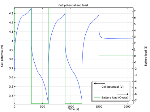
In the associated text field, type Cell potential (V).
|
|
8
|
|
9
|
In the associated text field, type Battery load (1).
|
|
10
|
|
1
|
|
2
|
|
3
|
Click OK.
|
|
4
|
|
5
|
|
1
|
|
2
|
|
3
|
|
4
|
Locate the Legends section. In the table, enter the following settings:
|
|
5
|
|
6
|
|
7
|
|
8
|
|
9
|
Click OK.
|
|
1
|
In the Model Builder window, expand the Results>Probe Plot Group 2 node, then click Probe Plot Group 2.
|
|
2
|
|
3
|
|
4
|
|
5
|
|
6
|
|
7
|
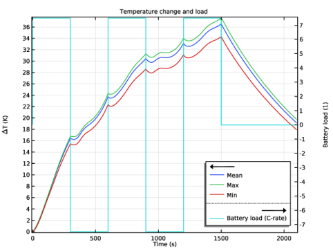
In the associated text field, type \DELTA T (K).
|
|
8
|
|
9
|
In the associated text field, type Battery load (1).
|
|
10
|
|
1
|
|
2
|
|
3
|
In the Columns list, choose T-T_inlet (K), Domain Probe 1, T-T_inlet (K), Domain Probe 2, and T-T_inlet (K), Domain Probe 3.
|
|
4
|
|
6
|
|
1
|
|
2
|
|
3
|
|
4
|
|
5
|
|
6
|
|
7
|
|
9
|
|
10
|
|
11
|
Click OK.
|
|
1
|
|
2
|
|
3
|
Click OK.
|
|
4
|
|
5
|
|
1
|
|
2
|
|
3
|
|
4
|
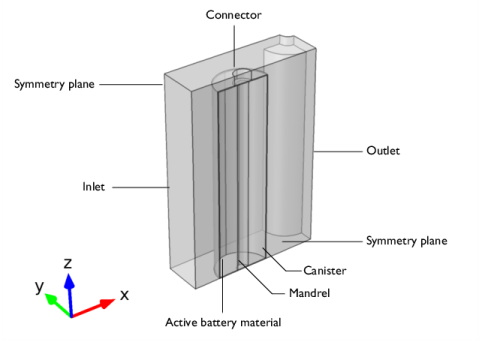
In the Add dialog box, in the Input selections list, choose Active Battery Material, Battery Connector, and Mandrel.
|
|
5
|
Click OK.
|
|
6
|
|
7
|
|
8
|
|
9
|
|
10
|
Click OK.
|
|
1
|
|
2
|
|
3
|
|
1
|
|
2
|
|
3
|
|
4
|
|
5
|
|
1
|
|
2
|
|
3
|
|
4
|
|
1
|
|
2
|
|
3
|
|
4
|
|
5
|
|
6
|
|
7
|
|
1
|
|
2
|
|
3
|
|
4
|
|
5
|
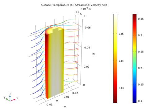
Click Replace Expression in the upper-right corner of the Expression section. From the menu, choose Component 2 (comp2)>Laminar Flow>Velocity and pressure>u,v,w - Velocity field.
|
|
6
|
Locate the Streamline Positioning section. From the Positioning list, choose On selected boundaries.
|
|
7
|
|
8
|
Locate the Coloring and Style section. Find the Line style subsection. From the Type list, choose Ribbon.
|
|
1
|
|
2
|
In the Settings window for Color Expression, click Replace Expression in the upper-right corner of the Expression section. From the menu, choose Component 2 (comp2)>Laminar Flow>Velocity and pressure>spf.U - Velocity magnitude - m/s.
|
|
3
|
|
4
|
|
1
|
|
2
|
|
3
|
Click OK.
|
|
1
|
|
2
|
|
3
|
Click OK.
|