|
|
|
|
•
|
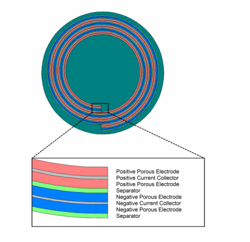
Two negative porous electrodes (60 μm thick)
|
|
•
|
Two positive porous electrodes (60 μm thick)
|
|
•
|
One negative current collector (14 μm thick)
|
|
•
|
One positive current collector (20 μm thick)
|
|
•
|
Two separator regions (30 μm thick)
|
|
1
|
|
2
|
|
3
|
Click Add.
|
|
4
|
Click
|
|
5
|
In the Select Study tree, select Preset Studies for Selected Physics Interfaces>Time Dependent with Initialization.
|
|
6
|
Click
|
|
1
|
|
2
|
|
3
|
|
4
|
Browse to the model’s Application Libraries folder and double-click the file li_battery_spiral_2d_parameters.txt.
|
|
1
|
|
2
|
|
3
|
|
4
|
|
5
|
|
6
|
|
1
|
|
2
|
|
3
|
|
1
|
|
2
|
|
3
|
|
4
|
|
5
|
|
6
|
|
1
|
|
2
|
|
3
|
|
4
|
|
5
|
|
1
|
|
2
|
|
3
|
|
4
|
|
5
|
|
1
|
|
2
|
|
3
|
|
4
|
|
5
|
|
1
|
|
2
|
|
3
|
|
4
|
|
5
|
|
1
|
|
2
|
|
3
|
|
4
|
|
5
|
|
1
|
|
2
|
|
3
|
|
4
|
|
5
|
|
1
|
|
2
|
|
3
|
|
4
|
|
5
|
|
1
|
|
2
|
|
3
|
|
4
|
|
5
|
|
6
|
|
1
|
|
2
|
Click in the Graphics window and then press Ctrl+A to select all objects.
|
|
3
|
|
1
|
|
2
|
|
3
|
|
4
|
|
5
|
|
6
|
|
1
|
|
2
|
|
1
|
|
2
|
|
1
|
|
2
|
|
1
|
|
2
|
|
1
|
|
2
|
|
1
|
|
2
|
|
3
|
|
1
|
|
2
|
|
3
|
|
1
|
|
2
|
|
1
|
|
2
|
|
3
|
|
4
|
In the Add dialog box, in the Selections to add list, choose Positive current collector, Negative current collector, Positive porous electrode, Negative porous electrode, and Electrolyte.
|
|
5
|
Click OK.
|
|
1
|
|
2
|
|
3
|
|
4
|
In the Add dialog box, in the Selections to add list, choose Positive porous electrode, Negative porous electrode, Electrolyte, and Electrolyte outside.
|
|
5
|
Click OK.
|
|
1
|
|
2
|
|
3
|
In the tree, select Built-in>Aluminum.
|
|
4
|
|
5
|
In the tree, select Built-in>Copper.
|
|
6
|
|
1
|
|
2
|
|
3
|
|
1
|
|
2
|
|
3
|
|
1
|
|
2
|
In the tree, select Battery>Electrolytes>LiPF6 in 1:2 EC:DMC and p(VdF-HFP) (Polymer electrolyte, Li-ion Battery).
|
|
3
|
|
4
|
|
5
|
|
6
|
|
7
|
|
8
|
|
1
|
In the Model Builder window, under Component 1 (comp1)>Materials click LiPF6 in 1:2 EC:DMC and p(VdF-HFP) (Polymer electrolyte, Li-ion Battery) (mat3).
|
|
2
|
|
3
|
|
1
|
In the Model Builder window, under Component 1 (comp1) right-click Lithium-Ion Battery (liion) and choose Porous Electrode.
|
|
2
|
|
3
|
|
4
|
Locate the Electrode Properties section. From the Electrode material list, choose Graphite Electrode, LixC6 MCMB (Negative, Li-ion Battery) (mat4).
|
|
5
|
|
6
|
|
1
|
In the Model Builder window, expand the Porous Electrode 1 node, then click Particle Intercalation 1.
|
|
2
|
|
3
|
From the Particle material list, choose Graphite Electrode, LixC6 MCMB (Negative, Li-ion Battery) (mat4).
|
|
4
|
|
5
|
|
6
|
|
1
|
|
2
|
|
3
|
|
4
|
|
5
|
|
6
|
|
1
|
|
2
|
|
3
|
|
4
|
Locate the Electrode Properties section. From the Electrode material list, choose LMO Electrode, LiMn2O4 Spinel (Positive, Li-ion Battery) (mat5).
|
|
5
|
|
6
|
|
1
|
In the Model Builder window, expand the Porous Electrode 2 node, then click Particle Intercalation 1.
|
|
2
|
|
3
|
From the Particle material list, choose LMO Electrode, LiMn2O4 Spinel (Positive, Li-ion Battery) (mat5).
|
|
4
|
|
5
|
|
6
|
|
1
|
|
2
|
|
3
|
|
4
|
|
5
|
|
6
|
|
1
|
|
2
|
|
3
|
|
1
|
|
2
|
|
3
|
|
1
|
|
2
|
|
3
|
|
1
|
|
2
|
In the Settings window for Electrode Current Density, type Electrode Current Density - 1C Discharge in the Label text field.
|
|
3
|
|
4
|
|
1
|
|
2
|
In the Settings window for Electrode Current Density, type Electrode Current Density - 10C Discharge in the Label text field.
|
|
3
|
|
4
|
|
5
|
|
6
|
|
7
|
|
8
|
|
1
|
|
1
|
|
2
|
|
3
|
|
1
|
|
1
|
|
2
|
|
3
|
|
1
|
|
1
|
|
2
|
|
3
|
|
1
|
|
1
|
|
2
|
|
3
|
|
1
|
|
1
|
|
2
|
|
3
|
|
4
|
In the Relative placement of vertices along edge text field, type 0 5e-5 10^range(-4,0.25,-2) range(2e-2,1e-2,0.98) (1-10^range(-2,-0.25,-4)) 0.99995 1.
|
|
1
|
|
2
|
|
3
|
|
4
|
|
1
|
|
2
|
|
1
|
|
2
|
|
3
|
|
4
|
Click Replace Expression in the upper-right corner of the Expression section. From the menu, choose Component 1 (comp1)>Lithium-Ion Battery>phis - Electric potential - V.
|
|
1
|
|
2
|
|
3
|
|
4
|
Locate the Physics and Variables Selection section. Select the Modify model configuration for study step check box.
|
|
5
|
In the Physics and variables selection tree, select Component 1 (comp1)>Lithium-Ion Battery (liion)>Electrode Current Density - 10C Discharge.
|
|
6
|
Click
|
|
7
|
|
8
|
|
9
|
|
1
|
|
2
|
|
3
|
|
1
|
|
2
|
|
3
|
|
1
|
|
2
|
|
3
|
|
1
|
|
2
|
|
3
|
|
1
|
|
2
|
|
3
|
|
4
|
|
5
|
|
6
|
|
7
|
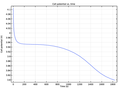
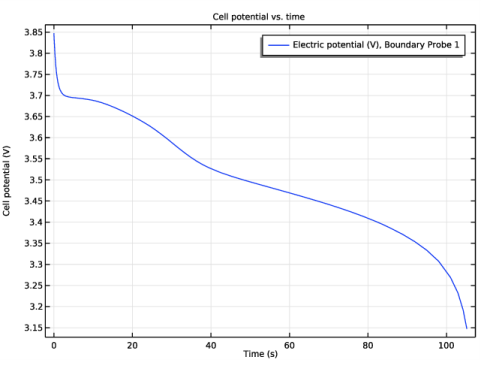
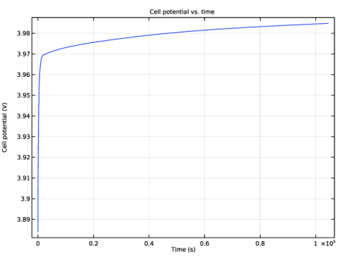
In the associated text field, type Cell potential (V).
|
|
8
|
|
1
|
|
2
|
|
3
|
|
4
|
|
1
|
|
2
|
|
3
|
|
4
|
|
1
|
|
2
|
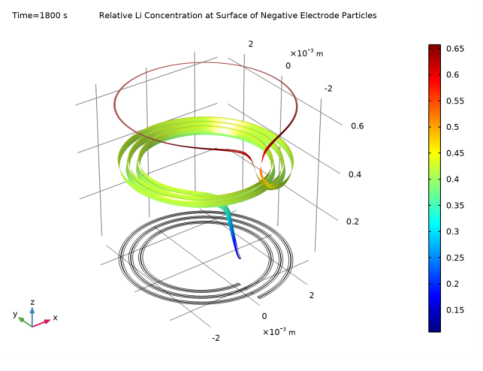
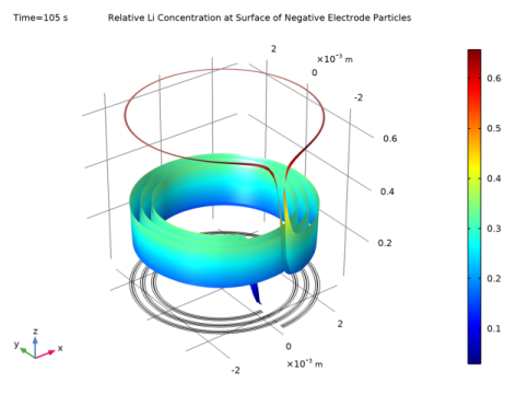
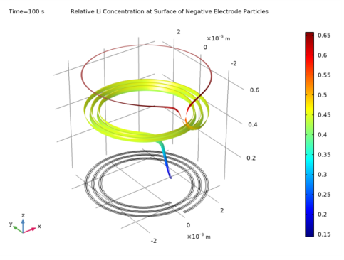
In the Settings window for 2D Plot Group, type Relative Li Concentration at Surface of Negative Electrode Particles in the Label text field.
|
|
3
|
|
4
|
Locate the Data section. From the Dataset list, choose Study 1 - 1 C Discharge/Solution 1 (4) (sol1).
|
|
1
|
Right-click Relative Li Concentration at Surface of Negative Electrode Particles and choose Surface.
|
|
2
|
In the Settings window for Surface, click Replace Expression in the upper-right corner of the Expression section. From the menu, choose Component 1 (comp1)>Lithium-Ion Battery>Particle intercalation>liion.socloc_surface - Local electrode material state-of-charge, particle surface.
|
|
1
|
|
2
|
|
1
|
|
2
|
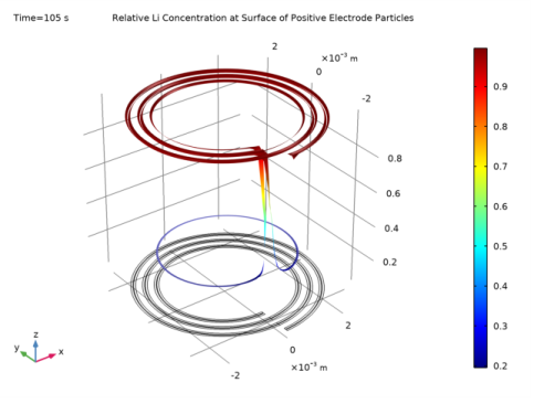
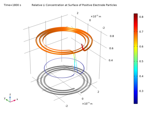
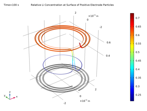
In the Settings window for 2D Plot Group, type Relative Li Concentration at Surface of Positive Electrode Particles in the Label text field.
|
|
3
|
Locate the Data section. From the Dataset list, choose Study 1 - 1 C Discharge/Solution 1 (5) (sol1).
|
|
4
|
|
1
|
Right-click Relative Li Concentration at Surface of Positive Electrode Particles and choose Surface.
|
|
2
|
In the Settings window for Surface, click Replace Expression in the upper-right corner of the Expression section. From the menu, choose Component 1 (comp1)>Lithium-Ion Battery>Particle intercalation>liion.socloc_surface - Local electrode material state-of-charge, particle surface.
|
|
1
|
|
2
|
|
1
|
|
2
|
|
3
|
Find the Studies subsection. In the Select Study tree, select Preset Studies for Selected Physics Interfaces>Time Dependent with Initialization.
|
|
4
|
|
5
|
|
1
|
|
2
|
|
3
|
|
4
|
Locate the Physics and Variables Selection section. Select the Modify model configuration for study step check box.
|
|
5
|
In the Physics and variables selection tree, select Component 1 (comp1)>Lithium-Ion Battery (liion)>Electrode Current Density - 1C Discharge.
|
|
6
|
Click
|
|
7
|
|
8
|
|
9
|
|
10
|
|
1
|
|
2
|
|
3
|
|
4
|
|
1
|
|
2
|
|
3
|
|
4
|
|
5
|
|
1
|
In the Model Builder window, under Results>Datasets click Study 1 - 1 C Discharge/Solution 1 (4) (sol1).
|
|
2
|
|
3
|
|
1
|
In the Model Builder window, under Results>Datasets click Study 1 - 1 C Discharge/Solution 1 (5) (sol1).
|
|
2
|
|
3
|
|
1
|
In the Model Builder window, click Relative Li Concentration at Surface of Negative Electrode Particles.
|
|
2
|
|
3
|
|
4
|
|
1
|
In the Model Builder window, click Relative Li Concentration at Surface of Positive Electrode Particles.
|
|
2
|
|
3
|
|
1
|
|
2
|
|
3
|
|
4
|
|
5
|
|
1
|
|
2
|
|
3
|
Locate the Physics and Variables Selection section. Select the Modify model configuration for study step check box.
|
|
4
|
In the Physics and variables selection tree, select Component 1 (comp1)>Lithium-Ion Battery (liion)>Electrode Current Density - 1C Discharge.
|
|
5
|
Click
|
|
6
|
In the Physics and variables selection tree, select Component 1 (comp1)>Lithium-Ion Battery (liion)>Electrode Current Density - 10C Discharge.
|
|
7
|
Click
|
|
8
|
Click to expand the Values of Dependent Variables section. Find the Initial values of variables solved for subsection. From the Settings list, choose User controlled.
|
|
9
|
|
10
|
|
11
|
|
12
|
In the Settings window for Study, type Study 3 - Relaxation after 1C Discharge in the Label text field.
|
|
13
|
|
14
|
|
1
|
In the Model Builder window, under Results>Datasets click Study 2 - 10 C Discharge/Solution 3 (4) (sol3).
|
|
2
|
|
3
|
|
1
|
In the Model Builder window, under Results>Datasets click Study 2 - 10 C Discharge/Solution 3 (5) (sol3).
|
|
2
|
|
3
|
|
1
|
|
2
|
|
3
|
|
4
|
|
5
|
Click
|
|
1
|
|
2
|
|
3
|
|
4
|
|
1
|
|
2
|
|
1
|
In the Model Builder window, click Relative Li Concentration at Surface of Negative Electrode Particles.
|
|
2
|
|
3
|
Click
|
|
1
|
In the Model Builder window, click Relative Li Concentration at Surface of Positive Electrode Particles.
|
|
2
|
|
3
|