|
|
|

|
•
|
|
•
|
|
1
|
|
2
|
Right-click Component 1 (comp1)>Lithium-Ion Battery (liion) and choose Electrode>Charge-Discharge Cycling.
|
|
4
|
|
5
|
|
6
|
|
7
|
|
8
|
|
9
|
|
10
|
|
11
|
|
1
|
|
2
|
In the Settings window for Porous Electrode, click to expand the Dissolving-Depositing Species section.
|
|
3
|
Click
|
|
5
|
|
6
|
Click to expand the Film Resistance section. From the Film resistance list, choose Thickness and conductivity.
|
|
7
|
|
8
|
|
9
|
|
1
|
|
2
|
|
3
|
From the Eeq list, choose User defined. Locate the Electrode Kinetics section. From the iloc,expr list, choose User defined. In the associated text field, type I_SEI*(cycle_no>0). The I_SEI variable was already defined in the seed file. You find the definition on the Component 1>Definitions>Variables 1 node.
|
|
4
|
Locate the Stoichiometric Coefficients section. In the νLiθ text field, type -(t_factor-1). The t_factor parameter is used to speed up the capacity fade per simulated cycle. You can read more about how the parameter is defined in the model documentation above.
|
|
5
|
In the Stoichiometric coefficients for dissolving-depositing species: table, enter the following settings:
|
|
6
|
Click to expand the Heat of Reaction section. From the dEeq/dT list, choose User defined. This is just a cosmetic setting to avoid the Materials node reporting missing material properties. The Heat of Reaction settings are not used in the model.
|
|
1
|
|
2
|
|
3
|
|
1
|
|
2
|
In the Settings window for Current Distribution Initialization, locate the Physics and Variables Selection section.
|
|
3
|
|
4
|
In the Physics and variables selection tree, select Component 1 (comp1)>Lithium-Ion Battery (liion)>Porous Electrode 1>Porous Electrode Reaction 2.
|
|
5
|
Click
|
|
1
|
|
2
|
|
3
|
|
4
|
Click
|
|
6
|
|
7
|
|
8
|
|
9
|
|
10
|
Clear the Generate default plots check box. For this model we are not interested in the default plots.
|
|
11
|
|
1
|
|
2
|
|
3
|
|
4
|
|
1
|
|
2
|
|
1
|
|
2
|
|
3
|
|
1
|
|
2
|
|
3
|
|
4
|
|
5
|
|
1
|
|
2
|
|
3
|
|
4
|
|
5
|
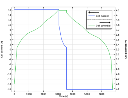
In the associated text field, type Cell potential (V).
|
|
1
|
|
2
|
|
3
|
|
4
|
|
5
|
|
1
|
|
2
|
|
3
|
|
1
|
|
2
|
|
3
|
|
1
|
|
2
|
|
3
|
|
4
|
|
1
|
|
2
|
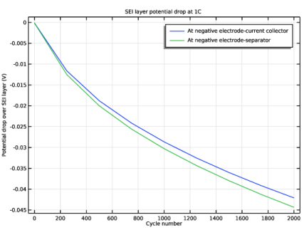
In the Settings window for 1D Plot Group, type SEI layer potential drop at 1C in the Label text field.
|
|
3
|
|
4
|
|
5
|
In the associated text field, type Potential drop over SEI layer (V).
|
|
1
|
|
3
|
|
4
|
|
5
|
|
6
|
|
7
|
Select the Description check box.
|
|
8
|
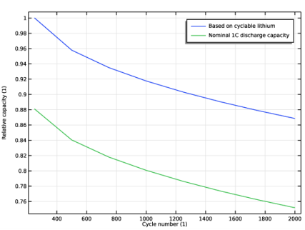
In the associated text field, type Cycle number.
|
|
9
|
|
10
|
|
1
|
|
2
|
|
3
|
|
1
|
In the Model Builder window, under Results>SEI layer potential drop at 1C right-click Point Graph 1 and choose Duplicate.
|
|
2
|
|
3
|
|
5
|
Locate the Legends section. In the table, enter the following settings:
|
|
6
|
|
1
|
|
2
|
|
3
|
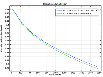
Locate the Plot Settings section. In the y-axis label text field, type Electrolyte volume fraction (1).
|
|
1
|
|
2
|
|
3
|
|
1
|
|
2
|
|
3
|
|
4
|
|
1
|
|
2
|
|
3
|
|
4
|
|
5
|
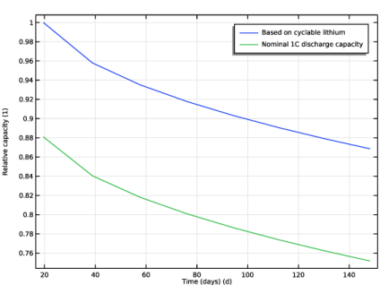
In the associated text field, type Time (days) (d).
|
|
6
|
|
7
|
In the associated text field, type Relative capacity (1).
|
|
1
|
|
2
|
|
4
|
|
5
|
|
6
|
Select the Description check box.
|
|
7
|
|
8
|
|
9
|
|
1
|
|
2
|
|
3
|
|
1
|
In the Model Builder window, under Results>Capacity vs. time right-click Global 1 and choose Duplicate.
|
|
2
|
|
4
|
Locate the Legends section. In the table, enter the following settings:
|
|
1
|
|
2
|
|
1
|
|
2
|
|
3
|
|
1
|
|
2
|
|
3
|
|
1
|
|
2
|
|
3
|
|
4
|
|
1
|
|
2
|
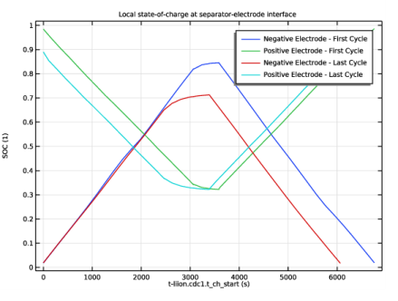
In the Settings window for 1D Plot Group, type Local state-of-charge at separator-electrode interface in the Label text field.
|
|
3
|
|
4
|
|
5
|
In the associated text field, type SOC (1).
|
|
1
|
|
3
|
|
4
|
|
5
|
Click to expand the Title section. Locate the x-Axis Data section. From the Parameter list, choose Expression.
|
|
6
|
|
7
|
|
8
|
|
1
|
|
2
|
|
3
|
|
1
|
In the Model Builder window, under Results>Local state-of-charge at separator-electrode interface right-click Point Graph 1 and choose Duplicate.
|
|
2
|
|
3
|
|
5
|
Locate the Legends section. In the table, enter the following settings:
|
|
1
|
|
2
|
|
1
|
|
2
|
|
3
|
|
1
|
In the Model Builder window, under Results>Local state-of-charge at separator-electrode interface right-click Point Graph 2 and choose Duplicate.
|
|
2
|
|
1
|
|
2
|
|
3
|
|
4
|