Transfer Impedance of a Perforate

Perforates are plates with a distribution of small perforations or holes. They are used in muffler systems, sound absorbing panels, and in many other places as liners, where it is important to control attenuation precisely. As the perforations become smaller and smaller, the viscous and thermal losses become more important. The attenuation behavior, which is also frequency dependent, can be controlled by selecting the perforate size and distribution in a plate. Nonlinear loss mechanisms occur at higher sound levels or in the presence of a flow (through/bias or over/grazing the perforate). Only the linear effects due to viscosity and thermal conduction are studied in this tutorial model. These effects are modeled in detail using the Thermoviscous Acoustics, Frequency Domain interface.

Perforates have been theoretically studied for many years. Typically, analytical or semi-analytical models only apply for simple geometries. A numerical approach is necessary for systems where the holes have various cross sections, if the perforations are tapered, or if the distribution of holes is uneven or of mixed sizes.

In this model, a simple perforate with circular holes is studied. The transfer impedance, surface normal impedance, and attenuation coefficient of the system is determined. The transfer impedance determined in this detailed model can, for example, be used in a larger system simulation using the interior impedance condition that exists in the Pressure Acoustics, Frequency Domain interface.

Model Definition

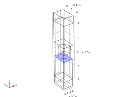
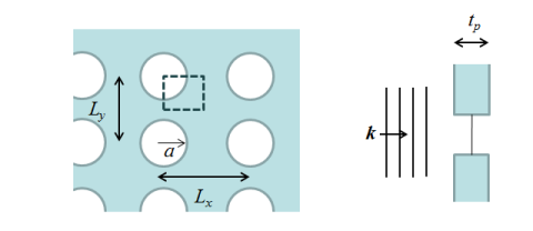
A sketch of the perforate system simulated is depicted in Figure 1. The model uses the symmetries that exist in the geometry along the x- and y-directions.

Figure 1: Schematic of the system, front and side views. The modeled region is marked by a box.

In Figure 1 the plate thickness is tp, the hole radius is named a, the hole-hole x and y distances are named Lx and Ly, respectively. In this model, the default values are tp = 1.0 mm, a = 0.5 mm, Lx = 1.4 mm, and Ly = 2.0 mm. A plane wave is incident from one side, modeled using the Background Acoustic Fields feature in the Thermoviscous Acoustics interface.

The transfer impedance Ztrans, surface normal impedance Zn, and absorption coefficient α are defined as

(1)

where Δp is the pressure drop across the plate, v is the mean velocity in the perforation hole, n is the surface normal of the perforate, and R is the reflection coefficient. These expressions are defined as variables in the model (imported from a file), under the node.

The transfer impedance of a perforate (perforated plate) is a well-studied problem in acoustics. Several models exist: some are pure analytical and some are semi-analytical. In this tutorial model, the results obtained in the simulation are compared to a semi-analytical expression for the transfer impedance Ztrans presented in Ref. 3 and Ref. 4. The expression combines an expression for the linear losses including viscosity (given in Ref. 1) and an expression for nonlinear effects at high levels (given in Ref. 2). The model also includes hole-hole interaction effects (semi-empirical). In this tutorial, the COMSOL model only consider linear acoustics. We include thermal and viscous losses as well as hole-hole interaction fully. In Equation 2, retaining the nonlinear term is out of interest and shows how it can be added to an analytical expression in COMSOL Multiphysics. The magnitude of that term is very small with the chosen levels. The semi-analytical model is given by the expression

(2)

where ρ0 is the fluid density, c0 the speed of sound, μ is the dynamic viscosity, Jn is the Bessel function of the first kind, ks is the shear (viscous) wave number, Urms the rms acoustic velocity in the hole, σ the porosity, and Cd is the discharge coefficient (a typical value is 0.76). Ψ is the so-called Fok function is defined by

(3)

The transfer impedance expression in Equation 2 does not include thermal effects. These can be added by modifying the linear part of the transfer impedance expression. The thermal effects are small for thin perforated plate (in the small k·tp limit) where shear and viscous losses dominate, see Ref. 5.

Results and Discussion

The total acoustic pressure in the system is depicted in Figure 2 evaluated at 2000 Hz. The acoustic particle velocity is depicted in Figure 3 at two different frequencies (400 and 2000 Hz). From the figure, the viscous boundary layer is easily seen as well as its frequency dependence (decreases with increasing frequency). Moreover, the end correction extent is also visualized here, as the part of the fluid moving axially, that extends out of the orifice. In Figure 4, the acoustic temperature variations can be seen. Here, as for the viscous boundary layer, the thermal boundary layer can be visualized.

Figure 2: Pressure distribution in the system.

Figure 3: Velocity distribution at 400 Hz and 2000 Hz.

Figure 4: Temperature distribution at 400 Hz and 2000 Hz.

The simulated value of the transfer impedance is depicted in Figure 5 and compared to the semi-analytical model given by Equation 2. The results are seen to coincide well. On the logarithmic y-axis scale, there is a constant difference between the curves. This corresponds to a factor multiplied on the linear scale. This could be due to the end correction and the hole-hole interaction modeled with the Fok function. In the present case, the holes are not equidistant in all directions. This can also make the simulation results deviate from the analytical assumptions.

The surface normal impedance experienced by a plane wave is depicted in Equation 6 and the absorption coefficient is depicted in Equation 7.

Finally, the instantaneous acoustic particle velocity is depicted using mirror data sets in the last Figure 8.

Figure 5: Transfer impedance as function of frequency. Comparing the COMSOL Multiphysics model results and the semianalytical expression.

Figure 6: Surface normal impedance of the perforated plate.

Figure 7: Absorption coefficient of the perforated plate.

Figure 8: Instantaneous velocity plotted using the symmetry data sets.

Notes About the COMSOL Implementation

Solver

This model does not use the default direct solver, but an iterative approach with a so-called direct preconditioner. This is one of the predefined iterative solver suggestions generated by COMSOL Multiphysics (it is then simply to enable it). This solver strategy is described in the Acoustics Module User’s Guide in the Modeling with Thermoviscous Acoustics section. The approach is ideal for medium sized pure thermoviscous acoustics models; the iterative solver is both faster and more memory efficient than the default direct solver.

The present model utilized the symmetries of the geometry to reduce the model size. Some perforated plate conflagrations may not have the same possibilities and thus require solving a larger problem. If the resulting problem becomes too large for the first iterative solver suggestion (used in this tutorial), the second iterative solver suggestion may be used. It is based on the domain decomposition (DD) method. This solver is very memory efficient but slower. An example can be found on the COMSOL homepage at:

•

www.comsol.com/model/transfer-impedance-of-a-perforate-12585

Mesh

When setting up the mesh, the parameter dvisc has been used as a measure of the viscous boundary layer thickness at the maximal study frequency. The viscous boundary layer thickness is given by

which at 100 Hz is equal to 0.22 mm for air. Thus the expression 220[um]*sqrt(100[Hz]/fmax) used in the parameter list for dvisc.

Reflection Coefficient

In the expression for the reflection coefficient R given under , the down() operator has been used in order to access the values of the background and scattered field variables on the side of the boundary where the feature is defined. The orientation up/down is relative to the surface normal which can be visualized with an arrow surface plot of the normal vector components nx, ny, and nz.

References

1. I. B. Crandall, “Theory of Vibrating Systems and Sound”, D. Van Nostrand Company, New York (1926).

2. T. H. Melling, “The acoustic impedance of perforates at medium and high sound pressure levels”, J. Sound Vibration 29, 1-65 (1973).

3. T. Schultz, F. Liu, L. Cattafesta, M. Sheplak, and M. Jones, “A Comparison Study of Normal-Incidence Acoustic Impedance Measurements of a Perforated Liner”, NASA Technical Reports Server LF99-801 (2009).

4. T. Schultz, F. Liu, L. Cattafesta, M. Sheplak, and M. Jones, “A Comparison Study of Normal-Incidence Acoustic Impedance Measurements of a Perforated Liner”, 15th AIAA/CEAS Aeroacoustics conference, AIAA 2009-3301.

5. A. W. Nolle, “Small-Signal Impedance of Short Tubes”, J. Acoust. Soc. Am. 25, 32-39 (1952).

Acoustics_Module/Tutorials,_Thermoviscous_Acoustics/transfer_impedance_perforate

Modeling Instructions

From the menu, choose .

New

In the window, click

Model Wizard

In the window, click

In the tree, select .

Click .

Click

In the tree, select .

Click

Global Definitions

Start by loading the global parameters that define the geometry and mesh parameters.

Parameters 1

In the window, under click .

In the window for , locate the section.

Click

Browse to the model’s Application Libraries folder and double-click the file transfer_impedance_perforate_parameters.txt.

Geometry 1

The next task is to set up the geometry of the perforate. The following instructions walk you through the steps of creating a fully parameterized geometry of one quarter of a hole as depicted in Figure 1. The instructions are quite lengthy.

If you want to skip these steps, the geometry sequence can be imported by right-clicking the node and selecting . Browse to your COMSOL installation folder under Multiphysics>applications>Acoustics_Module>Tutorials and select transfer_impedance_perforate.mph. After this, just continue setting up the model from the section below.

Cylinder 1 (cyl1)

In the toolbar, click

In the window for , locate the section.

In the text field, type a.

In the text field, type tp.

Locate the section. In the text field, type -tp/2.

Click to expand the section. Clear the check box.

Select the check box.

In the table, enter the following settings:


Layer name	Thickness (m)
Layer 1	tp/2

Block 1 (blk1)

In the toolbar, click

In the window for , locate the section.

In the text field, type Lx/2.

In the text field, type Ly/2.

In the text field, type Lz+Lpml.

Locate the section. In the text field, type tp/2.

Click to expand the section. Find the subsection. Clear the check box.

Select the check box.

In the table, enter the following settings:


Layer name	Thickness (m)
Layer 1	Lpml

Block 2 (blk2)

In the toolbar, click

In the window for , locate the section.

In the text field, type Lx/2.

In the text field, type Ly/2.

In the text field, type Lz+Lpml.

Locate the section. In the text field, type -(Lz+Lpml+tp/2).

Locate the section. In the table, enter the following settings:


Layer name	Thickness (m)
Layer 1	Lpml

Work Plane 1 (wp1)

In the toolbar, click

In the window for , locate the section.

From the list, choose .

Work Plane 2 (wp2)

In the toolbar, click

In the window for , locate the section.

From the list, choose .

Partition Objects 1 (par1)

In the toolbar, click

and choose .

Select the object only.

In the window for , locate the section.

From the list, choose .

Click

Partition Objects 2 (par2)

In the toolbar, click

and choose .

Select the object only.

In the window for , locate the section.

From the list, choose .

Click

Delete Entities 1 (del1)

In the window, right-click and choose .

In the window for , locate the section.

From the list, choose .

On the object , select Domains 1–6 only.

Click

Click the

button in the toolbar.

Definitions

Load the variables that define the transfer impedance, normal surface impedance, and absorption coefficient. The variables also define the semianalytical transfer impedance model defined in Equation 2.

Variables 1

In the window, expand the node.

Right-click and choose .

In the window for , locate the section.

Click

Browse to the model’s Application Libraries folder and double-click the file transfer_impedance_perforate_variables.txt.

Now, first set up integration operators on the two sides of the plate (in and out) as well as in the center of the tube (mid). Create selections for the symmetry planes and the wall. Finally, add the perfectly matched layers (PMLs) that truncate the computational domain.

Integration 1 (intop1)

In the toolbar, click

and choose .

Click the

button in the toolbar.

Click the

button in the toolbar.

In the window for , locate the section.

From the list, choose .

Select Boundaries 9 and 21 only.

It might be easier to select the boundaries by using the window. To open this window, in the toolbar click and choose . (If you are running the cross-platform desktop, you find in the main menu.)

In the text field, type intop_in.

Integration 2 (intop2)

In the toolbar, click

and choose .

In the window for , locate the section.

From the list, choose .

Select Boundaries 15 and 23 only.

In the text field, type intop_out.

Integration 3 (intop3)

In the toolbar, click

and choose .

In the window for , locate the section.

From the list, choose .

Select Boundary 12 only.

In the text field, type intop_mid.

Symmetry

In the toolbar, click

In the window for , type Symmetry in the text field.

Locate the section. From the list, choose .

Select the check box, to simplify selection and click on one face on each symmetry planes. Alternatively select the following faces.

Select Boundaries 1, 2, 4, 5, 7, 8, 10, 11, 13, 14, 16, 17, and 24–31 only.

Wall

In the toolbar, click

In the window for , type Wall in the text field.

Locate the section. From the list, choose .

Select Boundaries 20–23 only.

Perfectly Matched Layer 1 (pml1)

In the toolbar, click

Select Domains 1 and 6 only.

Materials

Add air as the material and set the bulk viscosity to 0.

Add Material

In the toolbar, click

to open the window.

Go to the window.

In the tree, select .

Click

In the toolbar, click

to close the window.

Proceed to set up the physics.

Thermoviscous Acoustics, Frequency Domain (ta)

Symmetry 1

In the window, under right-click and choose .

In the window for , locate the section.

From the list, choose .

Finally, add an incident plane wave using the feature with the option. Since the domain is backed by a PML, this configuration will allow reflections from the surface to leave the computational domain.

Background Acoustic Fields 1

In the toolbar, click