PDF

Topology Optimization and Verification of an Acoustic Mode in a 2D Room
Introduction
This tutorial introduces the use of topology optimization in acoustics. The goal of the optimization is to find the optimal material distribution (solid or air) in a given design domain, here the ceiling of a 2D room, that minimizes the average sound pressure level in an objective region. The optimization is carried out for a single frequency. The topology optimized design is further transformed into a geometry and the results of the optimization are verified using sound hard boundaries. See the tutorial Optimizing the Shape of a Horn for instructions on how to perform the optimization for a frequency band.
The model was inspired by the work of M. B. Dühring, O. Sigmund, and J. Søndergaard Jensen (Ref. 1).
Note: This application requires the Acoustics Module and the Optimization Module.
Figure 1: The initial design has a pressure node at the edge of the objective domain.
Model Definition
The room is exited with a monopole point source. The initial sound pressure level is shown in Figure 1. The objective is to minimize the average sound pressure level in the circular domain illustrated in the figure. The optimization is allowed to distribute material in the top of the room (a layer of the ceiling). The top domain is constrained to consists of at least 85 % air, but there are no other constraints, so the material does not have to connect with the top boundary.
The gradient-based optimization solver, in the Optimization Module, by default evaluates derivatives of the objective function via the solution of an adjoint equation. This procedure requires that the symbolic derivative of any nonanalytic function is selected in a special way. The default behavior of the composite functions abs(z) and conj(z), which are most commonly used to obtain a real-valued objective function, is to return a derivative parallel to the real axis. However, this behavior is not appropriate for the adjoint method, where you instead need the definitions
(1)
It is indeed possible to redefine the symbolic derivatives of built-in functions in COMSOL Multiphysics, but in this case it is more convenient to use the special function
realdot(z1,z2), which evaluates as real(z1·conj(z2)) but differentiates according to Equation 1.
The model uses the Density Model feature to solve the topology optimization problem using the density method. This means that the geometry is defined implicitly using non-physical material parameters. The local value of a given material parameter is determined by the local value of a control variable field, θc, which is bounded between zero and one, zero corresponding to some solid material and one to air.
Within the field of acoustic topology optimization it is common to interpolate the inverse density and bulk modulus linearly, that is,
(2)
where ρ1 and K1 are the density and bulk modulus of aluminum, respectively, while ρ2 and K2 are the properties of air. Wherever θ is equal to one, the properties of air are thus used. θ is the material volume factor, which is related to the control variable field, θc, through a filtering and projection step; see the Topology Optimization of an MBB Beam model in the Optimization Module Application Library for details. Acoustic topology optimization can be sensitive to small design changes, which can easily occur during post-processing of the topology optimization results. To reduce these issues, a continuation strategy is applied in the projection slope β. The model thus solves a sequence of optimization problems starting from a low projection slope and initializing the optimization with higher values using the previous optimization results.
Results and Discussion
The topology optimization achieves a large reduction of the average sound pressure level in the objective domain by moving a pressure node into the domain. The topology optimization result is further transferred to a new component using a Filter dataset. In this step a solid geometry is generated from the optimized solution. This causes the node to shift a bit, but it still goes through the domain as shown in Figure 2.
Figure 2: The sound pressure level is plotted after the optimization result has been transfered to a new component utilizing sound hard boundaries.
The value of the objective function is computed for a range of frequencies for the initial design as well as the topology optimized design (both before and after the verification step). The graph is plotted in Figure 3. It shows that the objective is only improved in a narrow frequency band around the optimization frequency. The verification step does not seem to cause the objective function to change noticeably.
Figure 3: The objective function is plotted as a function of frequency for the initial and topology optimized designs.
Reference
1. M. B. Dühring, O. Sigmund, and J. S. Jensen, Optimization of acoustic, optical and optoelastic devices, Kgs. Lyngby, Denmark: Technical University of Denmark (DTU), DCAMM Special Report No. S109, 2009.
Application Library path: Acoustics_Module/Optimization/topology_optimization_2d_room
 
Modeling Instructions
From the File menu, choose New.
New
In the New window, click  Model Wizard.
Model Wizard
1
In the Model Wizard window, click  2D.
2
In the Select Physics tree, select Acoustics>Pressure Acoustics>Pressure Acoustics, Frequency Domain (acpr).
3
Click Add.
4
Click  Study.
5
In the Select Study tree, select General Studies>Frequency Domain.
6
Global Definitions
Parameters 1
You can type in the parameters listed below or load them from topology_optimization_2d_room_parameters.txt.
1
In the Model Builder window, under Global Definitions click Parameters 1.
2
In the Settings window for Parameters, locate the Parameters section.
3
Geometry 1
Rectangle 1 (r1)
1
In the Geometry toolbar, click  Rectangle.
2
In the Settings window for Rectangle, locate the Size and Shape section.
3
In the Width text field, type W.
4
In the Height text field, type H.
5
Click to expand the Layers section. In the table, enter the following settings:
6
Clear the Layers on bottom check box.
7
Select the Layers on top check box.
Circle 1 (c1)
1
In the Geometry toolbar, click  Circle.
2
In the Settings window for Circle, locate the Size and Shape section.
3
In the Radius text field, type Rob.
4
Locate the Position section. In the x text field, type xob.
5
In the y text field, type yob.
6
Locate the Selections of Resulting Entities section. Select the Resulting objects selection check box.
Point 1 (pt1)
1
In the Geometry toolbar, click  Point.
2
In the Settings window for Point, locate the Point section.
3
In the x text field, type 2.
4
In the y text field, type 2.
5
Locate the Selections of Resulting Entities section. Select the Resulting objects selection check box.
Form Union (fin)
1
In the Model Builder window, click Form Union (fin).
2
In the Settings window for Form Union/Assembly, click  Build Selected.
Design Domain
1
In the Geometry toolbar, click  Selections and choose Box Selection.
2
In the Settings window for Box Selection, type Design Domain in the Label text field.
3
Locate the Box Limits section. In the y minimum text field, type H-dH/2.
Pressure Acoustics, Frequency Domain (acpr)
Pressure Acoustics 1
1
In the Model Builder window, under Component 1 (comp1)>Pressure Acoustics, Frequency Domain (acpr) click Pressure Acoustics 1.
2
In the Settings window for Pressure Acoustics, locate the Pressure Acoustics Model section.
3
From the Specify list, choose Bulk modulus and density.
4
From the K list, choose User defined. In the associated text field, type K1*(1+alpha_K*i).
5
From the ρ list, choose User defined. In the associated text field, type rho1.
Monopole Point Source 1
1
In the Physics toolbar, click  Points and choose Monopole Point Source.
2
In the Settings window for Monopole Point Source, locate the Point Selection section.
3
From the Selection list, choose Point 1.
4
Locate the Point Source section. In the QS text field, type 0.02.
Mesh 1
Free Triangular 1
In the Mesh toolbar, click  Free Triangular.
Size 1
1
Right-click Free Triangular 1 and choose Size.
2
In the Settings window for Size, locate the Geometric Entity Selection section.
3
From the Geometric entity level list, choose Domain.
4
From the Selection list, choose Design Domain.
5
Click to expand the Element Size Parameters section. Locate the Element Size section. Click the Custom button.
6
Locate the Element Size Parameters section. Select the Maximum element size check box.
7
Size 2
1
In the Model Builder window, right-click Free Triangular 1 and choose Size.
2
In the Settings window for Size, locate the Geometric Entity Selection section.
3
From the Geometric entity level list, choose Point.
4
From the Selection list, choose Point 1.
5
Locate the Element Size section. Click the Custom button.
6
Locate the Element Size Parameters section. Select the Maximum element size check box.
7
Size
1
In the Model Builder window, click Size.
2
In the Settings window for Size, click to expand the Element Size Parameters section.
3
In the Maximum element size text field, type hmax.
4
Click  Build All.
Definitions
Objective Function
1
In the Definitions toolbar, click  Probes and choose Domain Probe.
2
In the Settings window for Domain Probe, type Objective Function in the Label text field.
3
In the Variable name text field, type obj.
4
Locate the Source Selection section. From the Selection list, choose Circle 1.
The realdot operator is analytic, so if we use this to define the probe, it can be used as objective function without enabling splitting of complex variables.
5
Locate the Expression section. In the Expression text field, type 0.5*realdot(p,p)/acpr.pref_SPL^2.
Study 1
Step 1: Frequency Domain
1
In the Model Builder window, under Study 1 click Step 1: Frequency Domain.
2
In the Settings window for Frequency Domain, locate the Study Settings section.
3
Click  Range.
4
In the Range dialog box, type 24 in the Start text field.
5
In the Step text field, type 0.1.
6
In the Stop text field, type 42.
7
Click Replace.
8
In the Settings window for Frequency Domain, click to expand the Results While Solving section.
9
From the Probes list, choose None.
10
In the Model Builder window, click Study 1.
11
In the Settings window for Study, type Study 1 - Initial Design in the Label text field.
12
Locate the Study Settings section. Select the Generate default plots check box.
13
In the Home toolbar, click  Compute.
Results
Acoustic Pressure (acpr)
1
In the Settings window for 2D Plot Group, locate the Data section.
2
From the Parameter value (freq (Hz)) list, choose 34.5.
3
In the Acoustic Pressure (acpr) toolbar, click  Plot.
Sound Pressure Level (acpr)
1
In the Model Builder window, click Sound Pressure Level (acpr).
2
In the Settings window for 2D Plot Group, locate the Data section.
3
From the Parameter value (freq (Hz)) list, choose 34.5.
4
In the Sound Pressure Level (acpr) toolbar, click  Plot.
5
Click the  Zoom Extents button in the Graphics toolbar.
Acoustic Pressure (acpr), Sound Pressure Level (acpr)
1
In the Model Builder window, under Results, Ctrl-click to select Acoustic Pressure (acpr) and Sound Pressure Level (acpr).
2
Study 1 - Initial Design
In the Settings window for Group, type Study 1 - Initial Design in the Label text field.
Definitions
Setup the topology optimization by adding a Density Model and interpolate the inverse density and inverse bulk modulus linearly.
Density Model 1 (dtopo1)
1
In the Definitions toolbar, click  Optimization and choose Density Model.
2
In the Settings window for Density Model, locate the Geometric Entity Selection section.
3
From the Selection list, choose Design Domain.
4
Locate the Projection section. From the Projection type list, choose Hyperbolic tangent projection.
5
In the β text field, type beta.
6
Locate the Interpolation section. From the Interpolation type list, choose Linear.
7
Locate the Control Variable Initial Value section. In the θ0 text field, type volfrac.
Design Domain Variables
1
In the Model Builder window, right-click Definitions and choose Variables.
2
In the Settings window for Variables, type Design Domain Variables in the Label text field.
3
Locate the Geometric Entity Selection section. From the Geometric entity level list, choose Domain.
4
From the Selection list, choose Design Domain.
5
Locate the Variables section. In the table, enter the following settings:
Pressure Acoustics, Frequency Domain (acpr)
Pressure Acoustics (Design Domain)
1
In the Physics toolbar, click  Domains and choose Pressure Acoustics.
2
In the Settings window for Pressure Acoustics, type Pressure Acoustics (Design Domain) in the Label text field.
3
Locate the Domain Selection section. From the Selection list, choose Design Domain.
4
Locate the Pressure Acoustics Model section. From the Specify list, choose Bulk modulus and density.
5
From the K list, choose User defined. In the associated text field, type Kd_inv*(1+alpha_K*i).
6
From the ρ list, choose User defined. In the associated text field, type rhod_inv.
Disable the feature in the 1st study.
Study 1 - Initial Design
Step 1: Frequency Domain
1
In the Model Builder window, under Study 1 - Initial Design click Step 1: Frequency Domain.
2
In the Settings window for Frequency Domain, locate the Physics and Variables Selection section.
3
Select the Modify model configuration for study step check box.
4
In the Physics and variables selection tree, select Component 1 (comp1)>Pressure Acoustics, Frequency Domain (acpr)>Pressure Acoustics (Design Domain).
5
Click  Disable.
Add Study
1
In the Home toolbar, click  Add Study to open the Add Study window.
2
Go to the Add Study window.
3
Find the Studies subsection. In the Select Study tree, select General Studies>Frequency Domain.
4
Click Add Study in the window toolbar.
5
In the Home toolbar, click  Add Study to close the Add Study window.
Study 2
Step 1: Frequency Domain
1
In the Settings window for Frequency Domain, locate the Study Settings section.
2
In the Frequencies text field, type f0.
Topology Optimization
1
In the Model Builder window, right-click Study 2 and choose Optimization>Topology Optimization.
2
In the Settings window for Topology Optimization, locate the Optimization Solver section.
3
In the Maximum number of iterations text field, type 40.
4
Click Add Expression in the upper-right corner of the Objective Function section. From the menu, choose Component 1 (comp1)>Definitions>comp1.obj - Objective Function.
5
Locate the Objective Function section. In the table, enter the following settings:
6
Click Add Expression in the upper-right corner of the Constraints section. From the menu, choose Component 1 (comp1)>Definitions>Density Model 1>Global>comp1.dtopo1.theta_avg - Average material volume factor.
7
Locate the Constraints section. In the table, enter the following settings:
8
Locate the Output While Solving section. From the Probes list, choose None.
Initialize the study to generate a plot for use while solving.
9
In the Study toolbar, click  Get Initial Value.
Results
Acoustic Pressure (acpr) 1, Sound Pressure Level (acpr) 1
In the Model Builder window, under Results, Ctrl-click to select Acoustic Pressure (acpr) 1 and Sound Pressure Level (acpr) 1.
Acoustic Pressure (acpr) 1, Sound Pressure Level (acpr) 1
In the Model Builder window, under Results, Ctrl-click to select Acoustic Pressure (acpr) 1 and Sound Pressure Level (acpr) 1.
Study 2 - Topology Optimization
1
In the Model Builder window, under Results click Topology Optimization.
2
In the Settings window for Group, type Study 2 - Topology Optimization in the Label text field.
Surface 1
1
In the Model Builder window, expand the Threshold node, then click Surface 1.
2
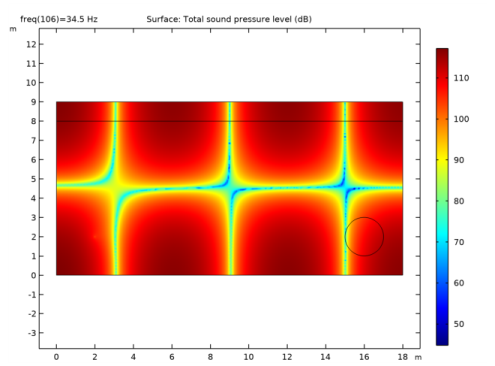
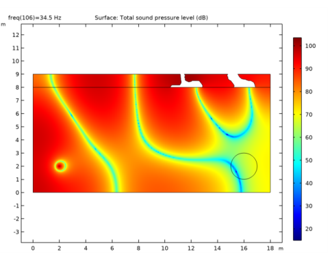
In the Settings window for Surface, click Replace Expression in the upper-right corner of the Expression section. From the menu, choose Component 1 (comp1)>Pressure Acoustics, Frequency Domain>Pressure and sound pressure level>acpr.Lp_t - Total sound pressure level - dB.
3
Locate the Coloring and Style section. From the Coloring list, choose Color table.
Study 2
Topology Optimization
1
In the Model Builder window, under Study 2 click Topology Optimization.
2
In the Settings window for Topology Optimization, locate the Output While Solving section.
3
Select the Plot check box.
4
From the Plot group list, choose Threshold.
5
In the Model Builder window, click Study 2.
6
In the Settings window for Study, type Study 2 - Topology Optimization in the Label text field.
7
Locate the Study Settings section. Clear the Generate default plots check box.
Use a Parametric Sweep to perform continuation in the projection slope parameter beta.
Parametric Sweep
1
In the Study toolbar, click  Parametric Sweep.
2
In the Settings window for Parametric Sweep, locate the Study Settings section.
3
4
5
Locate the Output While Solving section. From the Probes list, choose None.
6
Click to expand the Advanced Settings section. Select the Reuse solution from previous step check box.
7
In the Study toolbar, click  Compute.
Root
Add a study to generate the spectrum for the topology optimized design.
Add Study
1
In the Study toolbar, click  Add Study to open the Add Study window.
2
Go to the Add Study window.
3
Find the Studies subsection. In the Select Study tree, select General Studies>Frequency Domain.
4
Click Add Study in the window toolbar.
5
In the Study toolbar, click  Add Study to close the Add Study window.
Study 3
Step 1: Frequency Domain
1
In the Settings window for Frequency Domain, locate the Results While Solving section.
2
From the Probes list, choose None.
3
Click to expand the Values of Dependent Variables section. Find the Initial values of variables solved for subsection. From the Settings list, choose User controlled.
4
From the Method list, choose Solution.
5
From the Study list, choose Study 2 - Topology Optimization, Frequency Domain.
6
Locate the Study Settings section. Click  Range.
7
In the Range dialog box, type 24 in the Start text field.
8
In the Step text field, type 0.1.
9
In the Stop text field, type 42.
10
Click Replace.
11
In the Model Builder window, click Study 3.
12
In the Settings window for Study, type Study 3 - Optimized Spectrum in the Label text field.
13
Locate the Study Settings section. Clear the Generate default plots check box.
14
In the Study toolbar, click  Compute.
Results
Add a 1D Plot Group to visualize the objective function as a function of the frequency.
Response Comparison
1
In the Home toolbar, click  Add Plot Group and choose 1D Plot Group.
2
In the Settings window for 1D Plot Group, type Response Comparison in the Label text field.
3
Click to expand the Title section. From the Title type list, choose Manual.
4
In the Title text area, type SPL in Objective Domain.
Global 1
1
Right-click Response Comparison and choose Global.
2
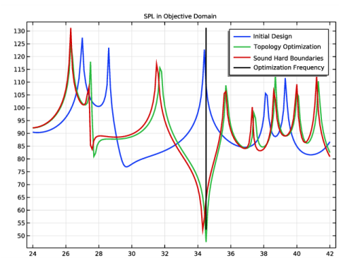
In the Settings window for Global, click Add Expression in the upper-right corner of the y-Axis Data section. From the menu, choose Component 1 (comp1)>Definitions>obj - Objective Function.
3
Locate the y-Axis Data section. In the table, enter the following settings:
4
Click to expand the Coloring and Style section. In the Width text field, type 2.
Global 2
1
Right-click Global 1 and choose Duplicate.
2
In the Settings window for Global, locate the Data section.
3
From the Dataset list, choose Study 3 - Optimized Spectrum/Solution 8 (sol8).
4
Locate the y-Axis Data section. In the table, enter the following settings:
Add a 2nd component with sound hard boundaries to verify that the optimization result can be trusted.
Filter
The exported geometry becomes smoother, if the filtered material volume factor is used instead of the (projected) material volume factor.
1
In the Model Builder window, expand the Results>Datasets node, then click Filter.
2
In the Settings window for Filter, locate the Evaluation section.
3
From the Smoothing list, choose Inside material domains.
4
Select the Use derivatives check box.
5
6
Right-click Results>Datasets>Filter and choose Create Mesh Part.
Mesh Part 1
Import 1
1
In the Settings window for Import, locate the Import section.
2
Click Import.
3
Click  Build All.
4
In the Model Builder window, right-click Mesh Part 1 and choose Create Geometry from Mesh.
Add Physics
1
In the Home toolbar, click  Add Physics to open the Add Physics window.
2
Go to the Add Physics window.
3
In the tree, select Acoustics>Pressure Acoustics>Pressure Acoustics, Frequency Domain (acpr).
4
Find the Physics interfaces in study subsection. In the table, clear the Solve check boxes for Study 1 - Initial Design, Study 2 - Topology Optimization, and Study 3 - Optimized Spectrum.
5
Click Add to Component 2 in the window toolbar.
6
In the Home toolbar, click  Add Physics to close the Add Physics window.
Pressure Acoustics, Frequency Domain 2 (acpr2)
Pressure Acoustics 1
1
In the Model Builder window, under Component 2 (comp2)>Pressure Acoustics, Frequency Domain 2 (acpr2) click Pressure Acoustics 1.
2
In the Settings window for Pressure Acoustics, locate the Pressure Acoustics Model section.
3
From the Specify list, choose Bulk modulus and density.
4
From the K list, choose User defined. In the associated text field, type K1*(1+alpha_K*i).
5
From the ρ list, choose User defined. In the associated text field, type rho1.
Monopole Point Source 1
1
In the Physics toolbar, click  Points and choose Monopole Point Source.
2
In the Settings window for Monopole Point Source, locate the Point Selection section.
3
From the Selection list, choose Point 1 (Import 1).
4
Locate the Point Source section. In the QS text field, type 0.02.
Mesh 2
Free Triangular 1
In the Mesh toolbar, click  Free Triangular.
Size 1
1
Right-click Free Triangular 1 and choose Size.
2
In the Settings window for Size, locate the Geometric Entity Selection section.
3
From the Geometric entity level list, choose Point.
4
From the Selection list, choose Point 1 (Import 1).
5
Locate the Element Size section. Click the Custom button.
6
Locate the Element Size Parameters section. Select the Maximum element size check box.
7
Size
1
In the Model Builder window, click Size.
2
In the Settings window for Size, locate the Element Size Parameters section.
3
In the Maximum element size text field, type hmax.
4
Click  Build All.
Definitions (comp2)
Objective Function
1
In the Definitions toolbar, click  Probes and choose Domain Probe.
2
In the Settings window for Domain Probe, type Objective Function in the Label text field.
3
In the Variable name text field, type obj.
4
Locate the Source Selection section. From the Selection list, choose Circle 1 (Import 1).
5
Locate the Expression section. In the Expression text field, type 0.5*realdot(p2,p2)/acpr2.pref_SPL^2.
Add Study
1
In the Home toolbar, click  Add Study to open the Add Study window.
2
Go to the Add Study window.
3
Find the Studies subsection. In the Select Study tree, select General Studies>Frequency Domain.
4
Find the Physics interfaces in study subsection. In the table, clear the Solve check box for Pressure Acoustics, Frequency Domain (acpr).
5
Click Add Study in the window toolbar.
6
In the Model Builder window, click the root node.
7
In the Home toolbar, click  Add Study to close the Add Study window.
Study 4
Step 1: Frequency Domain
1
In the Settings window for Frequency Domain, locate the Results While Solving section.
2
From the Probes list, choose None.
3
Locate the Study Settings section. Click  Range.
4
In the Range dialog box, type 24 in the Start text field.
5
In the Step text field, type 0.1.
6
In the Stop text field, type 42.
7
Click Replace.
8
In the Model Builder window, click Study 4.
9
In the Settings window for Study, type Study 4 - Verification in the Label text field.
10
In the Home toolbar, click  Compute.
Results
Topology Optimization
In the Model Builder window, under Results right-click Topology Optimization and choose Delete.
Acoustic Pressure (acpr2), Sound Pressure Level (acpr2)
1
In the Model Builder window, under Results, Ctrl-click to select Acoustic Pressure (acpr2) and Sound Pressure Level (acpr2).
2
Study 4 - Verification
In the Settings window for Group, type Study 4 - Verification in the Label text field.
Acoustic Pressure (acpr2)
1
In the Model Builder window, click Acoustic Pressure (acpr2).
2
In the Settings window for 2D Plot Group, locate the Data section.
3
From the Parameter value (freq (Hz)) list, choose 34.5.
4
In the Acoustic Pressure (acpr2) toolbar, click  Plot.
Sound Pressure Level (acpr2)
1
In the Model Builder window, click Sound Pressure Level (acpr2).
2
In the Settings window for 2D Plot Group, locate the Data section.
3
From the Parameter value (freq (Hz)) list, choose 34.5.
4
In the Sound Pressure Level (acpr2) toolbar, click  Plot.
5
Click the  Zoom Extents button in the Graphics toolbar.
Global 3
1
In the Model Builder window, under Results>Response Comparison right-click Global 2 and choose Duplicate.
2
In the Settings window for Global, locate the Data section.
3
From the Dataset list, choose Study 4 - Verification/Solution 9 (7) (sol9).
4
Locate the y-Axis Data section. In the table, enter the following settings:
The transition to sound hard boundaries causes the spectrum to shift slightly. Plot the position of the optimization frequency to see that this results in a slightly higher objective function.
Global 4
1
Right-click Global 3 and choose Duplicate.
2
In the Settings window for Global, locate the y-Axis Data section.
3
4
Locate the x-Axis Data section. From the Parameter list, choose Expression.
5
In the Expression text field, type f0.
6
Locate the Coloring and Style section. From the Color list, choose Black.
7
In the Response Comparison toolbar, click  Plot.
8
Click the  Zoom Extents button in the Graphics toolbar.