PDF

Optimizing the Shape of a Horn
Introduction
This example shows how to apply boundary shape optimization to a simple axisymmetric horn. For the sake of simplicity, the far-field sound pressure level is maximized for a single frequency and in a single direction. The focus is on the optimization procedure, which involves choice of objective function, and optimization solver settings. The deformation of the geometry is introduced using the Shape Optimization functionality of COMSOL Multiphysics.
The model was inspired by the work of Erik Bängtsson, Daniel Noreland, and Martin Berggren (Ref. 1).
Note: This application requires the Acoustics Module and the Optimization Module.
Figure 1: The initial configuration is a simple cone (the z<0 part of the gray area) in an infinite baffle.
Model Definition
A plane-wave mode feeds an axisymmetric horn radiating from an infinite baffle toward an open half space; see Figure 1. The radius of the feeding waveguide is assumed to be fixed, as well as the depth of the horn and the size of the hole where the horn is attached to the baffle. By varying the curvature of the initially conical surface of the horn, its directivity and impedance can be changed.
The surface is parameterized assuming that the radius and the z position of the horn deviates from the simple cone by a set of 8th-order Bernstein polynomials. The maximum displacement (in the two directions) is given by the dmax parameter. The number of optimization variables is determined by the order of the polynomial. Using a higher order gives more freedom and potentially a better final value of the objective function, but it also makes the optimization process more sensitive and can generate a shape that is less suitable for production.
Optimization can only be applied to real-valued functions because the minimum of a complex-valued function is not well-defined. But the raw result from a frequency-domain acoustics simulation is a complex-valued pressure field. From this you generate a scalar, real-valued quantity to be used as the objective function in the optimization process. However, any operation which converts a complex number to a real value is necessarily non-analytical, which means that its derivative is not uniquely defined.
The gradient-based optimization solver in the Optimization Module by default evaluates derivatives of the objective function via the solution of an adjoint equation. This procedure requires that the symbolic derivative of any non-analytic function is selected in a special way. The default behavior of the composite functions abs(z) and conj(z), which are most commonly used to obtain a real-valued objective function, is to return a derivative parallel to the real axis. However, this behavior is not appropriate for the adjoint method, where you instead need the definitions
(1)
It is indeed possible to redefine the symbolic derivatives of built-in functions in COMSOL Multiphysics, but in this case it is more convenient to use the special function realdot(z1z2), which evaluates as real(z1·conj(z2)) but differentiates according to Equation 1. In particular, as a measure of the transmission properties of the horn, use an expression of the form realdot(pmpm)/p02, where pm is the pressure measured at a specific point in front of the horn and p0 is the (real-valued and constant) amplitude of the incoming wave.
If you choose to evaluate pm in the near-field, or can afford to include a sufficiently large domain in front of the horn to effectively measure a far-field value at a point in the model, you can simply measure pm as the local pressure in a geometry vertex. However, in order to optimize the directivity pattern in an efficient way, pm should be defined using an integral representation of the exterior-field pressure as a function of the angle from the axis. Typically, for speaker it will be the pressure or SPL evaluated at a 1 m distance.
COMSOL Multiphysics contains optimized code for evaluating such exterior field integrals. This is, however, a pure postprocessing feature that does not support the automatic differentiation required by the adjoint method. Therefore, return to the definition of the Helmholtz-Kirchhoff integral as given in its axisymmetric form. See the Theory Background for the Pressure Acoustics Module section in the Acoustics Module User’s Guide for further details. To simplify things we will use the expression of the exterior field in the far-field limit.
(2)
If the infinite baffle is placed at z = 0, its effect is the same as that of adding a mirror image of the horn and at the same time removing the baffle. If, in addition, the integration surface is taken to be the wide end of the horn, in the plane of the baffle, most of the terms in Equation 2 cancel out, and all that is left is
(3)
where J0 is the Bessel function of the first kind of order 0, is the far-field evaluation distance, and the angle θ from the axis has been introduced as a parameter. This integral is easily implemented in COMSOL Multiphysics using an integration operator.
In this way the metric for the optimization is based on the far-field limit of the exterior field, which is valid for distances larger than the Rayleigh radius given by
Optimization as a rule implies many evaluations of the model for different designs, which can be very time consuming. In addition, the solver can be asked to evaluate each design at a number of frequencies and optimize with respect to the sum of the objective function values for each frequency. In this tutorial, a single frequency of 5000 Hz has been selected in order to make it possible to experiment with other aspects of the model. For example, changing the parameter θ, you can easily study the effect on the horn shape of optimizing the output at a specified angle from the axis.
Results and Discussion
By changing the shape of the horn within the limits of the selected parameterization, the on-axis sound pressure level can be raised by about 1 dB compared to the simple cone in Figure 1.
Figure 2: The final shape of the horn, optimized for on-axis SPL at 5000 Hz.
The improvement is rather small, because the initial design also shows a marked directivity, as can be seen from Figure 3. Obviously, the optimal shape with respect to on-axis SPL leads to deep undesirable minima in other directions.
Figure 3: Radiation plot of the original (dashed blue) and final (solid black) designs.
Optimizing with respect to a slight off-axis direction can give you a more uniform far-field pattern, but may also result in a deep minimum on the axis. Try for example to set the off-axis angle θ to 22° (in the parameters list set theta equal to 22[deg]).
Varying the frequency reveals that the on-axis improvement is robust over a wide frequency band; see Figure 4.
Figure 4: The objective function is plotted as a function of the frequency for the initial as well as the optimized design.
To search for a stable and practically useful horn design, you might instead create a composite objective function as a weighted sum of transmission values evaluated for a number of discrete directions, or choose to minimize the deviation from the mean SPL over a range of angles. In addition, you would also want to optimize with respect to more than one frequency, and experiment with different parameterizations.
Notes About the COMSOL Implementation
COMSOL Multiphysics implements the parameterization as a prescribed boundary displacement in the Moving Mesh feature. The mesh is allowed to move freely in the conical part of the horn, but otherwise kept fix. Some measures must be taken to avoid inverted elements when the shape of the cone is changed. Firstly, a quad mesh is used, since quads are less likely to become inverted, compared to triangles.
Secondly, the amplitude of the boundary displacement is restricted by the dmax parameter and the polynomial order. These constraints are intended to keep the mesh element volumes positive at all times and must not be active at the optimum point. You perform this sanity check as a final postprocessing step.
A time-harmonic Pressure Acoustics, Frequency Domain interface solves for the pressure field inside the horn and in a small spherical domain surrounding its opening. The air domain is terminated by a spherical PML layer which absorbs outgoing waves in such a way that the artificial termination of the domain has no influence on the near field. An accurate near field is sufficient, since the far-field result is based on an integral representation evaluated in the plane of the baffle. A plane wave radiation boundary condition on the waveguide attached to the narrow end of the horn feeds the horn with a plane wave of amplitude 1 Pa.
Set up the optimization problem in the Optimization study node. The pressure measured by an integration coupling variable, according to Equation 3, is inserted into a scalar objective function equal to the SPL value, or 10·log10(0.5·realdot(pmpm)/(20·106)2).
Reference
1. E. Bängtsson, D. Noreland, and M. Berggren, “Shape Optimization of an Acoustic Horn,” Technical Report 2002-019, Department of Information Technology, Uppsala University, May 2002.
Application Library path: Acoustics_Module/Optimization/horn_shape_optimization
Modeling Instructions
From the File menu, choose New.
New
In the New window, click  Model Wizard.
Model Wizard
1
In the Model Wizard window, click  2D Axisymmetric.
2
In the Select Physics tree, select Acoustics>Pressure Acoustics>Pressure Acoustics, Frequency Domain (acpr).
3
Click Add.
4
Click  Study.
5
In the Select Study tree, select General Studies>Frequency Domain.
6
Geometry 1
Square 1 (sq1)
1
In the Geometry toolbar, click  Square.
2
In the Settings window for Square, locate the Size section.
3
In the Side length text field, type 0.025.
4
Locate the Position section. In the z text field, type -0.2.
Circle 1 (c1)
1
In the Geometry toolbar, click  Circle.
2
In the Settings window for Circle, locate the Size and Shape section.
3
In the Radius text field, type 0.3.
4
In the Sector angle text field, type 90.
5
Click to expand the Layers section. In the table, enter the following settings:
6
Click  Build Selected.
7
Click the  Zoom Extents button in the Graphics toolbar.
Polygon 1 (pol1)
1
In the Geometry toolbar, click  Polygon.
2
In the Settings window for Polygon, locate the Coordinates section.
3
From the Data source list, choose Vectors.
4
In the r text field, type 0 0.1 0.1 0.025 0.025 0.
5
In the z text field, type 0 0 0 -0.175 -0.175 -0.175.
Global Definitions
Parameters 1
1
In the Model Builder window, under Global Definitions click Parameters 1.
2
In the Settings window for Parameters, locate the Parameters section.
3
Definitions
Integration 1 (intop1)
1
In the Definitions toolbar, click  Nonlocal Couplings and choose Integration.
2
In the Settings window for Integration, locate the Source Selection section.
3
From the Geometric entity level list, choose Boundary.
4
Variables 1
1
In the Definitions toolbar, click  Local Variables.
2
In the Settings window for Variables, locate the Variables section.
3
In the definition of pm, intop1() is the name of your integration operator, r is the radial coordinate, acpr.k is the local wave number, theta is the observation angle, and pz is the derivative of the pressure with respect to the z-coordinate.
Global Variable Probe 1 (var1)
1
In the Definitions toolbar, click  Probes and choose Global Variable Probe.
2
In the Settings window for Global Variable Probe, type obj in the Variable name text field.
3
Locate the Expression section. In the Expression text field, type 10*log10(0.5*realdot(pm,pm)/acpr.pref_SPL^2).
Perfectly Matched Layer 1 (pml1)
1
In the Definitions toolbar, click  Perfectly Matched Layer.
2
Now set up the shape optimization using a Free Shape Domain and a Polynomial Boundary feature.
Free Shape Domain 1
1
In the Definitions toolbar, click  Optimization and choose Free Shape Domain.
2
Polynomial Boundary 1
1
In the Definitions toolbar, click  Optimization and choose Polynomial Boundary.
2
3
In the Settings window for Polynomial Boundary, locate the Polynomial section.
4
In the n text field, type 8.
Add Material
1
In the Home toolbar, click  Add Material to open the Add Material window.
2
Go to the Add Material window.
3
4
Click Add to Component in the window toolbar.
5
In the Home toolbar, click  Add Material to close the Add Material window.
Pressure Acoustics, Frequency Domain (acpr)
Port 1
1
In the Model Builder window, under Component 1 (comp1) right-click Pressure Acoustics, Frequency Domain (acpr) and choose Port.
2
3
In the Settings window for Port, locate the Port Properties section.
4
From the Type of port list, choose Circular.
5
Locate the Incident Mode Settings section. In the Ain text field, type 1.
This gives you a plane wave with the amplitude 1 Pa propagating in the positive z direction
The default boundary condition is sound hard, which is appropriate for the horn surface and the baffle, and does no harm at the PML domain’s outer boundary. The PML and the incident plane-wave condition therefore fully specify the physics of the model. In order to prepare for the results processing, add an Exterior-Field Calculation node.
Exterior Field Calculation 1
1
In the Physics toolbar, click  Boundaries and choose Exterior Field Calculation.
2
3
In the Settings window for Exterior Field Calculation, locate the Exterior Field Calculation section.
4
From the Condition in the z = z^0 plane list, choose Symmetric/Infinite sound hard boundary.
5
From the Type of integral list, choose Far-field integral approximation for r-> infinity.
Mesh 1
Run the model at a frequency of 5 kHz, corresponding to a wavelength of just under 7 cm. Using the standard at-least-six-elements-per-wavelength rule, a maximum element size of 1 cm seems like a good choice. However, the shape wavelength along the edge of the cone should also be resolved, and the maximum wavelength is therefore set to 0.5 cm. A quad mesh is in general more resistant to element warping when the mesh is deformed. Therefore, use an unstructured quad mesh everywhere except in the PMLs, which perform better with a mapped mesh aligned with the radial and tangential directions.
Free Triangular 1
1
In the Mesh toolbar, click  Free Triangular.
2
In the Settings window for Free Triangular, locate the Domain Selection section.
3
From the Geometric entity level list, choose Domain.
4
Size
1
In the Model Builder window, click Size.
2
In the Settings window for Size, locate the Element Size section.
3
Click the Custom button.
4
Locate the Element Size Parameters section. In the Maximum element size text field, type 0.005.
Mapped 1
In the Mesh toolbar, click  Mapped.
Distribution 1
1
Right-click Mapped 1 and choose Distribution.
2
3
In the Settings window for Distribution, locate the Distribution section.
4
In the Number of elements text field, type 8.
5
Click  Build All.
Study 1 - Reference Solution
1
In the Model Builder window, click Study 1.
2
In the Settings window for Study, type Study 1 - Reference Solution in the Label text field.
Before starting the actual optimization, it is good practice to check the model setup by solving once with the default parameters. This way, you can also study the reference state on which you intend to improve.
Step 1: Frequency Domain
1
In the Model Builder window, under Study 1 - Reference Solution click Step 1: Frequency Domain.
2
In the Settings window for Frequency Domain, locate the Study Settings section.
3
In the Frequencies text field, type range(3500,50,6500).
4
Locate the Physics and Variables Selection section. In the table, clear the Solve for check box for Deformed geometry (Component 1).
5
In the Home toolbar, click  Compute.
Results
Acoustic Pressure, 3D (acpr)
The default plot in the main window shows the distribution of the instantaneous pressure in the physical domain and the PML. Note that the pressure near the outer boundary of the PML is practically zero. This has no physical relevance, but indicates that the PML is doing a good job absorbing the sound.
1
Click the  Zoom Extents button in the Graphics toolbar.
Probe Plot Group 8, Shape Optimization
1
In the Model Builder window, under Results, Ctrl-click to select Shape Optimization and Probe Plot Group 8.
2
Objective Validation
1
In the Home toolbar, click  Add Plot Group and choose 1D Plot Group.
2
In the Settings window for 1D Plot Group, type Objective Validation in the Label text field.
3
Click to expand the Title section. From the Title type list, choose Label.
4
Locate the Legend section. From the Position list, choose Upper left.
Global 1
1
Right-click Objective Validation and choose Global.
2
In the Settings window for Global, locate the y-Axis Data section.
3
4
Click Add Expression in the upper-right corner of the y-Axis Data section. From the menu, choose Component 1 (comp1)>Definitions>obj - Global Variable Probe 1.
5
In the Objective Validation toolbar, click  Plot.
Acoustic Pressure (acpr), Acoustic Pressure, 3D (acpr), Exterior-Field Pressure (acpr), Exterior-Field Sound Pressure Level (acpr), Objective Validation, Sound Pressure Level (acpr), Sound Pressure Level, 3D (acpr)
1
In the Model Builder window, under Results, Ctrl-click to select Acoustic Pressure (acpr), Sound Pressure Level (acpr), Acoustic Pressure, 3D (acpr), Sound Pressure Level, 3D (acpr), Exterior-Field Sound Pressure Level (acpr), Exterior-Field Pressure (acpr), and Objective Validation.
2
Reference solution
In the Settings window for Group, type Reference solution in the Label text field.
Root
Next, add a new study for the optimization.
Add Study
1
In the Home toolbar, click  Add Study to open the Add Study window.
2
Go to the Add Study window.
3
Find the Studies subsection. In the Select Study tree, select General Studies>Frequency Domain.
4
Click Add Study in the window toolbar.
5
In the Home toolbar, click  Add Study to close the Add Study window.
Study 2
Step 1: Frequency Domain
1
In the Settings window for Frequency Domain, locate the Study Settings section.
2
In the Frequencies text field, type f0-df/2 f0 f0+df/2.
3
In the Model Builder window, click Study 2.
4
In the Settings window for Study, type Study 2 - Optimized Solution in the Label text field.
Shape Optimization
1
Right-click Study 2 - Optimized Solution and choose Optimization>Shape Optimization.
2
In the Settings window for Shape Optimization, locate the Optimization Solver section.
3
Clear the Move limits check box.
4
Click Add Expression in the upper-right corner of the Objective Function section. From the menu, choose Component 1 (comp1)>Definitions>comp1.obj - Global Variable Probe 1.
Set up a MaxMin problems such that frequency associated with the worst objective function is prioritized.
5
Locate the Objective Function section. From the Type list, choose Maximization.
6
From the Solution list, choose Minimum of objectives.
Solution 2 (sol2)
1
In the Study toolbar, click  Show Default Solver.
By making the nonlinear tolerance stricter than that of the optimization solver, you ensure that the optimization does not fail because each solution is not sufficiently converged. An optimality tolerance of 1e-4 is still stricter than the accuracy of this low-resolution finite element model.
2
In the Model Builder window, expand the Solution 2 (sol2) node.
3
In the Model Builder window, expand the Study 2 - Optimized Solution>Solver Configurations>Solution 2 (sol2)>Optimization Solver 1 node, then click Stationary 1.
4
In the Settings window for Stationary, locate the General section.
5
In the Relative tolerance text field, type 1e-6.
6
From the Linearity list, choose Nonlinear.
7
In the Model Builder window, expand the Study 2 - Optimized Solution>Solver Configurations>Solution 2 (sol2)>Optimization Solver 1>Stationary 1 node, then click Fully Coupled 1.
8
In the Settings window for Fully Coupled, click to expand the Method and Termination section.
9
In the Minimum damping factor text field, type 1e-4.
10
Right-click Study 2 - Optimized Solution>Solver Configurations>Solution 2 (sol2)>Optimization Solver 1>Stationary 1>Fully Coupled 1 and choose Compute.
Results
Since the PML does not add any physical information it can be excluded for clarity.
Probe Solution 2 (sol2)
In the Model Builder window, expand the Results>Datasets node, then click Probe Solution 2 (sol2).
Selection
1
In the Results toolbar, click  Attributes and choose Selection.
2
In the Settings window for Selection, locate the Geometric Entity Selection section.
3
From the Geometric entity level list, choose Domain.
4
Acoustic Pressure (acpr) 1
The first default plot is the acoustic pressure. It should look like the image below.
Sound Pressure Level, 3D (acpr) 1
1
In the Model Builder window, click Sound Pressure Level, 3D (acpr) 1.
2
In the Sound Pressure Level, 3D (acpr) 1 toolbar, click  Plot.
Your plot of the sound pressure level should now look like Figure 2.
To see a direct comparison of the exterior-field polar pattern before and after optimization, modify the second to last default plot. This is an exterior-field plot of the sound pressure level in the rz-plane. Modify it to only plot the results in the positive half plane (z > 0), increase the resolution, and change some Coloring and Style options. The resulting plot of the exterior field should look like Figure 3. Note that 0 deg on the polar graph corresponds to the vertical z-axis.
Exterior-Field Pressure (acpr) 1
1
In the Model Builder window, click Exterior-Field Pressure (acpr) 1.
2
In the Settings window for Polar Plot Group, locate the Data section.
3
From the Parameter selection (freq) list, choose Manual.
4
In the Parameter indices (1-3) text field, type 2.
5
Click to expand the Title section. From the Title type list, choose Manual.
6
In the Title text area, type Exterior-field sound pressure level (dB).
Radiation Pattern 1
1
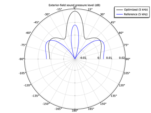
In the Model Builder window, expand the Exterior-Field Pressure (acpr) 1 node, then click Radiation Pattern 1.
2
In the Settings window for Radiation Pattern, locate the Evaluation section.
3
Find the Angles subsection. From the Restriction list, choose Manual.
4
In the φ start text field, type -90.
5
In the φ range text field, type 180.
6
Click to expand the Legends section. From the Legends list, choose Manual.
7
8
Click to expand the Coloring and Style section. From the Color list, choose Black.
Radiation Pattern 2
1
Right-click Results>Exterior-Field Pressure (acpr) 1>Radiation Pattern 1 and choose Duplicate.
2
In the Settings window for Radiation Pattern, locate the Data section.
3
From the Dataset list, choose Study 1 - Reference Solution/Solution 1 (sol1).
4
From the Parameter selection (freq) list, choose From list.
5
In the Parameter values (freq (Hz)) list, select 5000.
6
Locate the Legends section. In the table, enter the following settings:
7
Locate the Coloring and Style section. From the Color list, choose Blue.
8
In the Exterior-Field Pressure (acpr) 1 toolbar, click  Plot.
Acoustic Pressure (acpr) 1, Acoustic Pressure, 3D (acpr) 1, Exterior-Field Pressure (acpr) 1, Exterior-Field Sound Pressure Level (acpr) 1, Shape Optimization, Sound Pressure Level (acpr) 1, Sound Pressure Level, 3D (acpr) 1
1
In the Model Builder window, under Results, Ctrl-click to select Acoustic Pressure (acpr) 1, Sound Pressure Level (acpr) 1, Acoustic Pressure, 3D (acpr) 1, Sound Pressure Level, 3D (acpr) 1, Exterior-Field Sound Pressure Level (acpr) 1, Exterior-Field Pressure (acpr) 1, and Shape Optimization.
2
Optimized solution
In the Settings window for Group, type Optimized solution in the Label text field.
Add Study
1
In the Home toolbar, click  Add Study to open the Add Study window.
2
Go to the Add Study window.
3
Find the Studies subsection. In the Select Study tree, select General Studies>Frequency Domain.
4
Click Add Study in the window toolbar.
5
In the Home toolbar, click  Add Study to close the Add Study window.
Study 3
Step 1: Frequency Domain
1
In the Settings window for Frequency Domain, locate the Study Settings section.
2
In the Frequencies text field, type range(3500,50,6500).
3
Locate the Physics and Variables Selection section. In the table, clear the Solve for check box for Deformed geometry (Component 1).
4
Click to expand the Values of Dependent Variables section. Find the Values of variables not solved for subsection. From the Settings list, choose User controlled.
5
From the Method list, choose Solution.
6
From the Study list, choose Study 2 - Optimized Solution, Frequency Domain.
7
In the Model Builder window, click Study 3.
8
In the Settings window for Study, type Study 3 - Frequency Sweep (Optimized) in the Label text field.
9
Locate the Study Settings section. Clear the Generate default plots check box.
10
In the Home toolbar, click  Compute.
Results
Optimized solution
Add 1D Plot Group showing the objective function as a function of the frequency for the initial as well as the optimized design.
Response
1
In the Home toolbar, click  Add Plot Group and choose 1D Plot Group.
2
In the Settings window for 1D Plot Group, type Response in the Label text field.
3
Locate the Title section. From the Title type list, choose None.
4
Locate the Plot Settings section. Select the y-axis label check box.
5
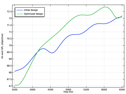
In the associated text field, type On axis SPL (objective).
6
Locate the Legend section. From the Position list, choose Upper left.
Global 1
1
Right-click Response and choose Global.
2
In the Settings window for Global, click Add Expression in the upper-right corner of the y-Axis Data section. From the menu, choose Component 1 (comp1)>Definitions>obj - Global Variable Probe 1.
3
Click to expand the Coloring and Style section. In the Width text field, type 2.
4
Click to expand the Legends section. From the Legends list, choose Manual.
5
Global 2
1
Right-click Global 1 and choose Duplicate.
2
In the Settings window for Global, locate the Data section.
3
From the Dataset list, choose Study 3 - Frequency Sweep (Optimized)/Solution 3 (sol3).
4
Locate the Legends section. In the table, enter the following settings:
Probe Plot Group 15
In the Model Builder window, right-click Probe Plot Group 15 and choose Delete.