PDF

Lumped Loudspeaker Driver Using a Lumped Mechanical System
Introduction
This is a model of a moving-coil loudspeaker where a lumped parameter analogy represents the behavior of the electrical and mechanical speaker components. This lumped model is coupled to a 2D axisymmetric pressure acoustics model describing the surrounding air domain.
This example illustrates an alternative way of modeling mechanical components (mass, spring, and damper) using the Lumped Mechanical System interface in a lumped loudspeaker driver model. More information regarding the theory and a model setup can be found in the model Lumped Loudspeaker Driver.
Note: This application requires the Acoustics Module, the AC/DC Module, the Structural Mechanics Module, and the Multibody Dynamics Module.
Model Definition
A schematic representation of a moving coil loudspeaker is given in Figure 1. The figure shows a cross section of a loudspeaker. The speaker driver is placed in an infinite baffle with free space in front and on the back of the speaker. The speaker cone consists of the outer suspension, the diaphragm, and a dust cap (not marked in the figure).
Figure 1: Schematic representation of a moving coil speaker unit.
The mechanical and electrical components of the speaker that are lumped are shown inside the dotted box. On the electrical side it includes the voice-coil and magnetic system (permanent magnet and pole pieces), and on the mechanical side it includes the moving mass of the voice coil and speaker cone, the spring effect of the spider and outer suspension, as well as possible losses due to damping in these suspensions.
Lumped Representation of Electrical and mechanical components
The lumped or circuit representation for the electrical and mechanical parts of the system sketched in Figure 1 is shown in Figure 2. The upper figure represents the voice coil electrical system and the lower figure represents the lumped mechanical system of the speaker cone, suspensions, and mass of the voice coil. In both figures the node numbers are also shown — they are very useful when setting up the circuit model in COMSOL.
Figure 2: The lumped (circuit) representation for the electrical (top) and mechanical (bottom) components of the speaker driver.
In Figure 2 (top) the external voltage source is denoted by V0 and the generator output resistance is Rg, in this model Rg = 0 Ω. The voice coil resistance is RE, and the voice coil inductance is LE(ω), which is frequency dependent. The losses in the magnetic circuit are modeled through the frequency dependent resistance R'E(ω). The current controlled voltage source BL·uD, represents the back induced electromagnetic voltage generated when the voice coil (of length L) moves with velocity uD in the magnetic field B. Here BL is the product of the magnetic field strength and the voice coil length L (see also Ref. 2 on how this can be modeled). In the electrical circuit the current is denoted ic.
The mechanical system given in Figure 2 (bottom) has the following components:
Mass (MMD) representing the mass of voice coil and diaphragm assembly
Spring (1/CMS) representing the stiffness of speaker suspensions (both spider and outer suspension)
Damping (RMS) representing the possible losses in suspensions
The speaker diaphragm is subjected to the following forces acting in the axial direction:
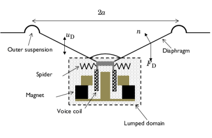
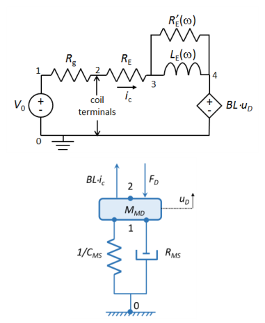
Lorentz force: The Lorentz force is given by BL·ic for a voice coil of length L with current ic, where B is the magnetic flux density.
(1)
where Δp is the pressure drop across the diaphragm and nz is the axial component of the surface normal n (see Figure 1). This expression gives the couplings from the acoustic finite element model to the lumped mechanical model. On the other hand, the coupling from the lumped mechanical model to the finite element model comes from specifying the acceleration on the surface of the diaphragm.
For more details about the model including small signal parameters, and finite element modeling refer to Ref. 3.
Results and Discussion
The generated pressure field is shown in Figure 3 for 1 kHz and 5 kHz. This plot shows the directive characteristic of the speaker cone at increasing frequencies, this nature is discussed more at the end of this section when discussing the directivity plot in Figure 7.
Figure 3: Acoustic pressure for a frequency of 1 kHz (top) and kHz (bottom).
Figure 4: The frequency dependent acoustic radiated power (upper left), electric input power (upper right), efficiency (lower left), and on-axis pressure field (lower right).
The first two graphs in Figure 4 (upper left and upper right) represent the acoustically radiated power PAR and the electric input power PE.
The third (lower-left) graph of Figure 4 represents the driver efficiency given in percent (%), that is, the ratio of the acoustic radiated power and the input electric power.
The pressure field along the z-axis is shown in the last graph of Figure 4 from z = Rair to z = 5 m, evaluated at a frequency of 1000 Hz. In the model a Parameterized Curve 2D is used to evaluate the exterior-field pressure outside the computational mesh.
Figure 5: The frequency dependent mechanical force amplitude (upper left), corresponding phase (upper right), diaphragm velocity amplitude (lower left), and corresponding phase (lower right).
In the top row of Figure 5 the frequency variation of the mechanical forces in mass, spring, and damper components are shown. The left graph shows the force amplitude whereas on the right graph, the phase is plotted. It can be seen that the spring force is dominant at low frequencies whereas the inertial force starts to dominate at higher frequencies. In the bottom row of Figure 5 the frequency variation of the amplitude and phase of the speaker cone axial velocity is shown.
The pressure and the sound pressure level evaluated at 1 m, using the dedicated radiation pattern plots, are shown in Figure 6, here evaluated at 10 kHz. In the figure the 0° mark corresponds to the axial z direction. Both figures show a very strong directive pattern as expected at this high frequency.
Figure 6: Exterior-field pressure and sound pressure level evaluated at a distance of 1 m the half sphere in front of the speaker and at 10 kHz.
In Figure 7 (top) the radiated intensity is illustrated which is evaluated at 100 Hz. The color plot represents the magnitude of the intensity vector I, the domain vector field represents the components of the intensity vector, and finally the vectors plotted on the edges represent the surface normals.
The final plot of this model is shown in Figure 7 (bottom), it is a so-called directivity plot of the speaker unit. The plot represents a contour plot of the sound pressure level Lp evaluated along a half circle in front of the speaker as function of the angle and the frequency, that is, Lp(θ, f). As this plot is a more advanced and nonstandard plot in COMSOL the axis labels are a bit off. The x-axis represents the angle and actually runs from 90° to 90°. The y-axis is a logarithmic frequency axis running from 101 Hz to 104 Hz. The plot illustrates how the spatial response goes from a nearly omnidirectional constant value at the low frequencies, through a single lobe response at intermediate frequencies, and ends up as a complex directive pattern at high frequencies. This type of plot is very often used, in industry, to characterize speakers and speaker units.
Figure 7: Top: intensity magnitude (color plot), intensity vector field (domain arrows), and surface normals (edge arrows) for 100 Hz. Bottom: directivity plot for the speaker. The x-axis is a scaled azimuthal angle that runs from -90° to 90° and the y-axis is a logarithmic frequency axis that runs from 10 Hz to 10 kHz.
References
1. W. Marshall Leach, Jr., Introduction to Electroacoustics and Audio Amplifier Design, Kendall Hunt, 2010.
2. Loudspeaker Driver Model Documentation, from the COMSOL Application Library.
3. Lumped Loudspeaker Driver Model Documentation, from the COMSOL Application Library.
Application Library path: Acoustics_Module/Electroacoustic_Transducers/lumped_loudspeaker_driver_mechanical
Modeling Instructions
From the File menu, choose New.
New
In the New window, click  Model Wizard.
Model Wizard
1
In the Model Wizard window, click  2D Axisymmetric.
2
In the Select Physics tree, select Acoustics>Pressure Acoustics>Pressure Acoustics, Frequency Domain (acpr).
3
Click Add.
4
In the Select Physics tree, select AC/DC>Electrical Circuit (cir).
5
Click Add.
6
In the Select Physics tree, select Structural Mechanics>Lumped Mechanical System (lms).
7
Click Add.
8
Click  Study.
9
In the Select Study tree, select General Studies>Frequency Domain.
10
Global Definitions
Load small signal and geometric parameters from a file.
Parameters 1
1
In the Model Builder window, under Global Definitions click Parameters 1.
2
In the Settings window for Parameters, locate the Parameters section.
3
Click  Load from File.
4
Import a simple 2D axisymmetric geometry of the speaker driver.
Geometry 1
Import 1 (imp1)
1
In the Home toolbar, click  Import.
2
In the Settings window for Import, locate the Import section.
3
Click Browse.
4
5
Click Import.
6
In the Home toolbar, click  Build All.
Now, set up all the variables, selections, and component couplings under the Definitions node.
Definitions
Model variables
1
In the Home toolbar, click  Variables and choose Local Variables.
2
In the Settings window for Variables, type Model variables in the Label text field.
3
Locate the Variables section. Click  Load from File.
4
Speaker
1
In the Definitions toolbar, click  Explicit.
2
In the Settings window for Explicit, type Speaker in the Label text field.
3
Locate the Input Entities section. From the Geometric entity level list, choose Boundary.
4
Internal wall
1
In the Definitions toolbar, click  Explicit.
2
In the Settings window for Explicit, type Internal wall in the Label text field.
3
Locate the Input Entities section. From the Geometric entity level list, choose Boundary.
4
Integration 1 (intop1)
1
In the Definitions toolbar, click  Nonlocal Couplings and choose Integration.
2
In the Settings window for Integration, locate the Source Selection section.
3
From the Geometric entity level list, choose Boundary.
4
From the Selection list, choose Speaker.
5
In the Operator name text field, type intop.
Perfectly Matched Layer 1 (pml1)
1
In the Definitions toolbar, click  Perfectly Matched Layer.
2
3
In the Settings window for Perfectly Matched Layer, locate the Scaling section.
4
From the Coordinate stretching type list, choose Rational.
5
In the PML scaling factor text field, type 0.5.
6
In the PML scaling curvature parameter text field, type 5.
You have now changed the default settings for the perfectly matched layer (PML). The new settings will improve the performance of the PML at very low frequencies.
Add Material
1
In the Home toolbar, click  Add Material to open the Add Material window.
2
Go to the Add Material window.
3
4
Click Add to Component in the window toolbar.
5
In the Home toolbar, click  Add Material to close the Add Material window.
Now, set up the physics and the boundary conditions for the model.
Pressure Acoustics, Frequency Domain (acpr)
Interior Sound Hard Boundary (Wall) 1
1
In the Model Builder window, under Component 1 (comp1) right-click Pressure Acoustics, Frequency Domain (acpr) and choose Interior Conditions>Interior Sound Hard Boundary (Wall).
2
In the Settings window for Interior Sound Hard Boundary (Wall), locate the Boundary Selection section.
3
From the Selection list, choose Internal wall.
Interior Normal Acceleration 1
1
In the Physics toolbar, click  Boundaries and choose Interior Normal Acceleration.
2
In the Settings window for Interior Normal Acceleration, locate the Boundary Selection section.
3
From the Selection list, choose Speaker.
4
Locate the Interior Normal Acceleration section. Specify the a0 vector as
Exterior Field Calculation 1
1
In the Physics toolbar, click  Boundaries and choose Exterior Field Calculation.
2
3
In the Settings window for Exterior Field Calculation, locate the Exterior Field Calculation section.
4
From the Condition in the z = z^0 plane list, choose Symmetric/Infinite sound hard boundary.
Proceed to set up the electric circuit system and lumped mechanical system part of the model. When building this look at Figure 2 for the references to the node numbers used in the model.
Electrical Circuit (cir)
In the Model Builder window, under Component 1 (comp1) click Electrical Circuit (cir).
Voltage Source 1 (V1)
1
In the Electrical Circuit toolbar, click  Voltage Source.
2
In the Settings window for Voltage Source, locate the Node Connections section.
3
4
Locate the Device Parameters section. In the vsrc text field, type V0.
Resistor 1 (R1)
1
In the Electrical Circuit toolbar, click  Resistor.
2
In the Settings window for Resistor, locate the Node Connections section.
3
4
Locate the Device Parameters section. In the R text field, type R_g.
Resistor 2 (R2)
1
In the Electrical Circuit toolbar, click  Resistor.
2
In the Settings window for Resistor, locate the Node Connections section.
3
4
Locate the Device Parameters section. In the R text field, type R_E.
Inductor 1 (L1)
1
In the Electrical Circuit toolbar, click  Inductor.
2
In the Settings window for Inductor, locate the Node Connections section.
3
4
Locate the Device Parameters section. In the L text field, type L_E.
Resistor 3 (R3)
1
In the Electrical Circuit toolbar, click  Resistor.
2
In the Settings window for Resistor, locate the Node Connections section.
3
4
Locate the Device Parameters section. In the R text field, type Rp_E.
Voltage Source 2 (V2)
1
In the Electrical Circuit toolbar, click  Voltage Source.
2
In the Settings window for Voltage Source, locate the Node Connections section.
3
4
Locate the Device Parameters section. In the vsrc text field, type BL*lms.M1_v.
Lumped Mechanical System (lms)
In the Model Builder window, under Component 1 (comp1) click Lumped Mechanical System (lms).
Spring 1 (K1)
1
In the Physics toolbar, click  Global and choose Spring.
2
In the Settings window for Spring, locate the Node Connections section.
3
4
Locate the Component Parameters section. In the k text field, type 1/C_MS.
5
Locate the Results section. Find the Add the following to default results subsection. Clear the Displacement check box.
Damper 1 (C1)
1
In the Physics toolbar, click  Global and choose Damper.
2
In the Settings window for Damper, locate the Node Connections section.
3
4
Locate the Component Parameters section. In the c text field, type R_MS.
5
Locate the Results section. Find the Add the following to default results subsection. Clear the Displacement check box.
Mass 1 (M1)
1
In the Physics toolbar, click  Global and choose Mass.
2
In the Settings window for Mass, locate the Node Connections section.
3
4
Locate the Component Parameters section. In the m text field, type M_MD.
5
Locate the Results section. Find the Add the following to default results subsection. Clear the Displacement check box.
6
Select the Velocity check box.
Force Node 1 (frc1)
1
In the Physics toolbar, click  Global and choose Force Node.
2
In the Settings window for Force Node, locate the Node Connections section.
3
4
Locate the Terminal Parameters section. In the fp10 text field, type BL*cir.R2_i+F_D.
Now, build the mesh. It consists of a triangular mesh around the speaker and an extruded mesh in the PML region. In the boundary where the exterior-field is calculated, add a single boundary layer.
Mesh 1
Free Triangular 1
1
In the Mesh toolbar, click  Free Triangular.
2
In the Settings window for Free Triangular, locate the Domain Selection section.
3
From the Geometric entity level list, choose Domain.
4
Size
1
In the Model Builder window, click Size.
2
In the Settings window for Size, locate the Element Size section.
3
Click the Custom button.
4
Locate the Element Size Parameters section. In the Maximum element size text field, type 343[m/s]/fmax/8.
5
In the Minimum element size text field, type 343[m/s]/fmax/100.
Mapped 1
1
In the Mesh toolbar, click  Mapped.
2
In the Settings window for Mapped, click  Build All.
Boundary Layers 1
1
In the Mesh toolbar, click  Boundary Layers.
2
In the Settings window for Boundary Layers, locate the Domain Selection section.
3
From the Geometric entity level list, choose Domain.
4
5
Click to expand the Transition section. Clear the Smooth transition to interior mesh check box.
Boundary Layer Properties
1
In the Model Builder window, click Boundary Layer Properties.
2
3
In the Settings window for Boundary Layer Properties, locate the Boundary Layer Properties section.
4
In the Number of boundary layers text field, type 1.
5
From the Thickness of first layer list, choose Manual.
6
In the Thickness text field, type 343[m/s]/fmax/100.
7
Click  Build All.
Study 1
Step 1: Frequency Domain
1
In the Model Builder window, under Study 1 click Step 1: Frequency Domain.
2
In the Settings window for Frequency Domain, locate the Study Settings section.
3
Click  Range.
4
In the Range dialog box, choose ISO preferred frequencies from the Entry method list.
5
In the Start frequency text field, type 10.
6
In the Stop frequency text field, type 10000.
7
From the Interval list, choose 1/24 octave.
8
Click Replace.
9
In the Home toolbar, click  Compute.
Results
Acoustic Pressure (acpr)
First, look at the default plots. Investigate the 2D Sound Pressure Level (acpr) plot to verify the performance of the perfectly matched layer (PML). After doing this you can disable plotting in the PML region, which is unphysical. Secondly, look at the default exterior-field plots and make a few changes, before setting up a range of plots to investigate the loudspeaker driver performance.
Sound Pressure Level (acpr)
Look at the sound pressure level (SPL) plots at the frequencies of 10 kHz, 1 kHz, and 10 Hz. Note that the SPL decreases nearly 100 dB over the width of the thickness of the PML. This means that the outgoing waves are extremely damped.
1
In the Model Builder window, click Sound Pressure Level (acpr).
2
In the Settings window for 2D Plot Group, locate the Data section.
3
From the Parameter value (freq (Hz)) list, choose 1000.
4
In the Sound Pressure Level (acpr) toolbar, click  Plot.
5
From the Parameter value (freq (Hz)) list, choose 10.
6
In the Sound Pressure Level (acpr) toolbar, click  Plot.
Study 1/Solution 1 (sol1)
In the Model Builder window, expand the Results>Datasets node, then click Study 1/Solution 1 (sol1).
Selection
1
In the Results toolbar, click  Attributes and choose Selection.
2
In the Settings window for Selection, locate the Geometric Entity Selection section.
3
From the Geometric entity level list, choose Domain.
4
Acoustic Pressure (acpr)
1
In the Model Builder window, click Acoustic Pressure (acpr).
2
In the Settings window for 2D Plot Group, locate the Data section.
3
From the Parameter value (freq (Hz)) list, choose 1000.
4
In the Acoustic Pressure (acpr) toolbar, click  Plot.
5
Click the  Zoom Extents button in the Graphics toolbar.
6
From the Parameter value (freq (Hz)) list, choose 5000.
7
In the Acoustic Pressure (acpr) toolbar, click  Plot.
These two plots should reproduce Figure 3.
Radiation Pattern 1
1
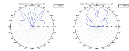
In the Model Builder window, expand the Exterior-Field Sound Pressure Level (acpr) node, then click Radiation Pattern 1.
2
In the Settings window for Radiation Pattern, locate the Evaluation section.
3
Find the Angles subsection. From the Restriction list, choose Manual.
4
In the φ start text field, type -90.
5
In the φ range text field, type 180.
6
In the Exterior-Field Sound Pressure Level (acpr) toolbar, click  Plot.
Radiation Pattern 1
1
In the Model Builder window, expand the Exterior-Field Pressure (acpr) node, then click Radiation Pattern 1.
2
In the Settings window for Radiation Pattern, locate the Evaluation section.
3
Find the Angles subsection. From the Restriction list, choose Manual.
4
In the φ start text field, type -90.
5
In the φ range text field, type 180.
6
In the Exterior-Field Pressure (acpr) toolbar, click  Plot.
These two polar plots should reproduce Figure 6.
Now modify the default plots of the Lumped Mechanical System interface to reproduce Figure 5.
Mechanical Force, Amplitude
1
In the Model Builder window, under Results click Force, Amplitude (lms) 1.
2
In the Settings window for 1D Plot Group, type Mechanical Force, Amplitude in the Label text field.
3
Click to expand the Title section. From the Title type list, choose Label.
4
Locate the Plot Settings section. In the y-axis label text field, type Force (N).
5
Locate the Legend section. From the Position list, choose Upper left.
6
Click the  x-Axis Log Scale button in the Graphics toolbar.
7
In the Mechanical Force, Amplitude toolbar, click  Plot.
Mechanical Force, Phase
1
In the Model Builder window, under Results click Force, Phase (lms) 1.
2
In the Settings window for 1D Plot Group, type Mechanical Force, Phase in the Label text field.
3
Locate the Title section. From the Title type list, choose Label.
4
Locate the Plot Settings section. In the y-axis label text field, type Phase (rad).
5
Locate the Legend section. From the Position list, choose Lower right.
6
Click the  x-Axis Log Scale button in the Graphics toolbar.
7
In the Mechanical Force, Phase toolbar, click  Plot.
Diaphragm Velocity, Amplitude
1
In the Model Builder window, under Results click Velocity, Amplitude (M1).
2
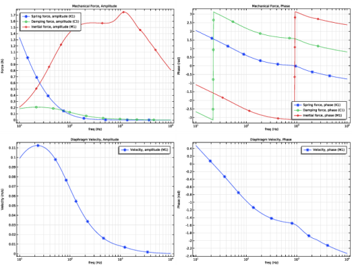
In the Settings window for 1D Plot Group, type Diaphragm Velocity, Amplitude in the Label text field.
3
Locate the Title section. From the Title type list, choose Label.
4
Locate the Plot Settings section. In the y-axis label text field, type Velocity (m/s).
5
Click the  x-Axis Log Scale button in the Graphics toolbar.
6
In the Diaphragm Velocity, Amplitude toolbar, click  Plot.
Diaphragm Velocity, Phase
1
In the Model Builder window, under Results click Velocity, Phase (M1).
2
In the Settings window for 1D Plot Group, type Diaphragm Velocity, Phase in the Label text field.
3
Locate the Title section. From the Title type list, choose Label.
4
Locate the Plot Settings section. In the y-axis label text field, type Phase (rad).
5
Click the  x-Axis Log Scale button in the Graphics toolbar.
6
In the Diaphragm Velocity, Phase toolbar, click  Plot.
Acoustic Radiated Power
1
In the Home toolbar, click  Add Plot Group and choose 1D Plot Group.
2
In the Settings window for 1D Plot Group, type Acoustic Radiated Power in the Label text field.
3
Locate the Title section. From the Title type list, choose Label.
4
Locate the Plot Settings section. Select the x-axis label check box.
5
6
Select the y-axis label check box.
7
8
Locate the Legend section. From the Position list, choose Lower middle.
Global 1
1
Right-click Acoustic Radiated Power and choose Global.
2
In the Settings window for Global, click Replace Expression in the upper-right corner of the y-Axis Data section. From the menu, choose Component 1 (comp1)>Definitions>Variables>P_AR - Radiated power - W.
3
In the Acoustic Radiated Power toolbar, click  Plot.
4
Click the  x-Axis Log Scale button in the Graphics toolbar.
This plot should reproduce Figure 4 (top left).
Electric Input Power
1
In the Home toolbar, click  Add Plot Group and choose 1D Plot Group.
2
In the Settings window for 1D Plot Group, type Electric Input Power in the Label text field.
3
Locate the Title section. From the Title type list, choose Label.
4
Locate the Plot Settings section. Select the x-axis label check box.
5
6
Select the y-axis label check box.
7
8
Locate the Legend section. From the Position list, choose Lower right.
Global 1
1
Right-click Electric Input Power and choose Global.
2
In the Settings window for Global, click Replace Expression in the upper-right corner of the y-Axis Data section. From the menu, choose Component 1 (comp1)>Definitions>Variables>P_E - Electric input power (rms) - W.
3
In the Electric Input Power toolbar, click  Plot.
4
Click the  x-Axis Log Scale button in the Graphics toolbar.
This plot should reproduce Figure 4 (top right).
Driver Efficiency
1
In the Home toolbar, click  Add Plot Group and choose 1D Plot Group.
2
In the Settings window for 1D Plot Group, type Driver Efficiency in the Label text field.
3
Locate the Title section. From the Title type list, choose Label.
4
Locate the Plot Settings section. Select the x-axis label check box.
5
6
Select the y-axis label check box.
7
Global 1
1
Right-click Driver Efficiency and choose Global.
2
In the Settings window for Global, locate the y-Axis Data section.
3
4
In the Driver Efficiency toolbar, click  Plot.
5
Click the  x-Axis Log Scale button in the Graphics toolbar.
This plot should reproduce Figure 4 (bottom left).
Set up a parameterized curve used to evaluate the exterior-field outside of the computational mesh.
Parameterized Curve 2D 1
1
In the Results toolbar, click  More Datasets and choose Parameterized Curve 2D.
2
In the Settings window for Parameterized Curve 2D, locate the Expressions section.
3
In the z text field, type s*5[m]+(1-s)*Rair.
4
Select the Only evaluate globally defined expressions check box.
On-axis Pressure Field
1
In the Results toolbar, click  1D Plot Group.
2
In the Settings window for 1D Plot Group, type On-axis Pressure Field in the Label text field.
3
Locate the Data section. From the Dataset list, choose Parameterized Curve 2D 1.
4
Locate the Title section. From the Title type list, choose Label.
5
Locate the Plot Settings section. Select the x-axis label check box.
6
7
Select the y-axis label check box.
8
9
Locate the Data section. From the Parameter selection (freq) list, choose From list.
10
In the Parameter values (freq (Hz)) list, select 1000.
11
Locate the Legend section. Clear the Show legends check box.
Line Graph 1
1
Right-click On-axis Pressure Field and choose Line Graph.
2
3
In the Settings window for Line Graph, locate the y-Axis Data section.
4
In the Expression text field, type pext(r,z).
5
Locate the x-Axis Data section. From the Parameter list, choose Expression.
6
In the Expression text field, type z.
7
Click to expand the Quality section. From the Resolution list, choose Extra fine.
8
In the On-axis Pressure Field toolbar, click  Plot.
This plot should reproduce Figure 4 (bottom right).
Create a 2D intensity plot that includes the magnitude of the intensity vector acpr.I_rms as well as an arrow surface (vector field plot) of the intensity vector, with the components (acpr.Ir,acpr.Iz).
Intensity
1
In the Home toolbar, click  Add Plot Group and choose 2D Plot Group.
2
In the Settings window for 2D Plot Group, type Intensity in the Label text field.
Surface 1
1
Right-click Intensity and choose Surface.
2
In the Settings window for Surface, locate the Expression section.
3
In the Expression text field, type acpr.I_rms.
Arrow Surface 1
1
In the Model Builder window, right-click Intensity and choose Arrow Surface.
2
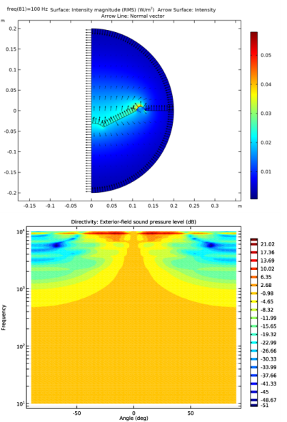
In the Settings window for Arrow Surface, click Replace Expression in the upper-right corner of the Expression section. From the menu, choose Component 1 (comp1)>Pressure Acoustics, Frequency Domain>Intensity>acpr.Ir,acpr.Iz - Intensity.
3
Locate the Coloring and Style section. From the Color list, choose Black.
Arrow Line 1
1
Right-click Intensity and choose Arrow Line.
2
In the Settings window for Arrow Line, click Replace Expression in the upper-right corner of the Expression section. From the menu, choose Component 1 (comp1)>Pressure Acoustics, Frequency Domain>Geometry>acpr.nr,acpr.nz - Normal vector.
3
Locate the Coloring and Style section. From the Color list, choose Black.
4
In the Intensity toolbar, click  Plot.
5
Click the  Zoom Extents button in the Graphics toolbar.
Now change the evaluation frequency to 5000 Hz, 1000 Hz, and 100 Hz in order to plot and reproduce Figure 7.
Intensity
1
In the Model Builder window, click Intensity.
2
In the Settings window for 2D Plot Group, locate the Data section.
3
From the Parameter value (freq (Hz)) list, choose 5000.
4
In the Intensity toolbar, click  Plot.
5
From the Parameter value (freq (Hz)) list, choose 1000.
6
In the Intensity toolbar, click  Plot.
7
From the Parameter value (freq (Hz)) list, choose 100.
8
In the Intensity toolbar, click  Plot.
Next create the directivity plot of the speaker.
Directivity
1
In the Home toolbar, click  Add Plot Group and choose 1D Plot Group.
2
In the Settings window for 1D Plot Group, type Directivity in the Label text field.
Directivity 1
1
In the Directivity toolbar, click  More Plots and choose Directivity.
2
In the Settings window for Directivity, locate the Evaluation section.
3
Find the Angles subsection. From the Restriction list, choose Manual.
4
In the φ start text field, type -90.
5
In the φ range text field, type 180.
6
Click to expand the Coloring and Style section. From the Layout list, choose Frequency on y-axis.
7
In the Directivity toolbar, click  Plot.
8
Click the  y-Axis Log Scale button in the Graphics toolbar.
This should reproduce the directivity plot depicted in Figure 7. You can tailor the plot to your needs using the normalization options or defining the specific levels to use in the contour plot.