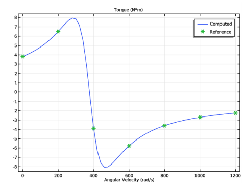
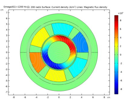
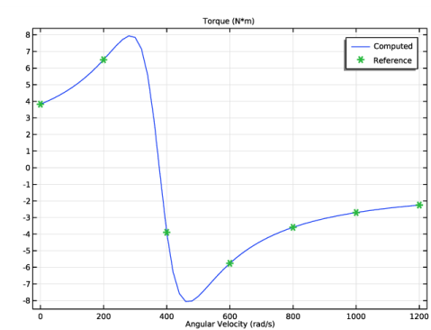
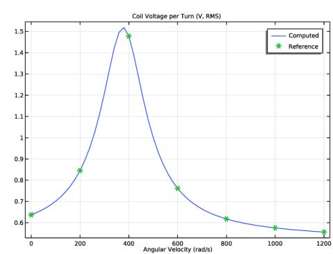
PDF

Frequency Domain Study of Three-Phase Motor
Introduction
This verification application is based on the first case detailed in the TEAM benchmark problem 30, “Induction Motor Analyses” (Ref. 1). The application performs a frequency domain analysis of a simple three-phase induction motor in 2D, with a circularly-symmetric rotor made of aluminum and iron. The solution is compared with analytic results; in particular, the torque, coil voltage, and losses are evaluated as functions of the rotational speed.
Model Definition
The model geometry is two-dimensional and is represented in Figure 1. This simplified geometry was chosen in Ref. 1 to allow computing the analytic solution to use as a reference for the numerical results.
Figure 1: Two-dimensional geometry of the three-phase induction motor.
The rotor consists of an iron core surrounded by an aluminum layer. The air gap and the region containing the six coils (windings), including the coil themselves, are nonmagnetic and nonconductive. The motor is surrounded by a layer of laminated iron and the outer region is air.
The rotating part is rotationally symmetric and it does not have magnetic sources (such as permanent magnets), so the rotation can be modeled by adding an artificial term (Lorentz’s term) to the constitutive relation for the conduction current:
(1)
where v is the local velocity of the material. The properties of the rotor and the constant rotational velocity ensure that all the fields and currents in the model are time-harmonic; so a frequency-domain analysis can be performed.
Using Lorentz’s term and a frequency-domain analysis allows setting up a numerical problem without the need for moving meshes, as it is normally done with the Rotating Machinery, Magnetic interface. The Magnetic Fields interface can be used instead. The Lorentz’s term is added by using a Velocity (Lorentz’s Term) feature.
The three-phase coils (windings) are modeled with three Coil features using the Homogenized multiturn conductor model, which provide a homogenized model of bundles of tiny conducting wires. The three Coils use the Coil group functionality to model the two series-connected phase groups with current flowing in opposite direction.
The quantities of interests, for which analytic data is provided in Ref, are:
Results and Discussion
Figure 2 and Figure 3 show the axial current density and the magnetic flux density lines for two different angular velocities, Ω = 200 rad/s and Ω = 800 rad/s, respectively, below and above the rotational velocity of the stator field (about 377 rad/s or 3600 RPM).
Figure 2: Axial current density and magnetic flux density lines for Ω = 200 rad/s.
Figure 3: Axial induced current density and magnetic flux density lines for Ω = 800 rad/s.
Since the analysis performed is in the frequency domain, the solutions plotted in Figure 2 and Figure 3 are the real part of the current density and magnetic flux density phasors. It is possible to visualize the evolution of the fields during a cycle by changing the value of the phase in the dataset or by creating an animation as demonstrated in the application.
Figure 4, Figure 5, and Figure 6 show the computed torque, the coil voltage, and the rotor losses as a function of the rotational velocity. The plots show the expected results for an induction motor; in particular, the torque is zero, the voltage is maximum, and the losses are at a minimum at the synchronous speed (Ω = 377 rad/s).
The computed solution shows very good agreement with the analytic data (green markers).
Figure 4: Computed (blue line) and analytic (green markers) torque as a function of the angular velocity of the rotor.
Figure 5: Computed (blue line) and analytic (green markers) coil voltage per turn as a function of the angular velocity of the rotor.
Figure 6: Computed (blue line) and analytic (green markers) rotor losses as a function of the angular velocity of the rotor.
Reference
1. http://www.compumag.org/jsite/team.html
Application Library path: ACDC_Module/Verification_Examples/three_phase_motor_frequency
Modeling Instructions
From the File menu, choose New.
New
In the New window, click  Model Wizard.
Model Wizard
1
In the Model Wizard window, click  2D.
2
In the Select Physics tree, select AC/DC>Electromagnetic Fields>Magnetic Fields (mf).
3
Click Add.
4
Click  Study.
5
In the Select Study tree, select General Studies>Frequency Domain.
6
Global Definitions
Parameters 1
1
In the Model Builder window, under Global Definitions click Parameters 1.
2
In the Settings window for Parameters, locate the Parameters section.
3
The geometry sequence is available in a separate file.
Geometry 1
1
In the Geometry toolbar, click  Insert Sequence.
2
3
In the Geometry toolbar, click  Build All.
4
Click the  Zoom Extents button in the Graphics toolbar.
Definitions
Integration, Steel
1
In the Definitions toolbar, click  Nonlocal Couplings and choose Integration.
2
3
In the Settings window for Integration, type Integration, Steel in the Label text field.
4
In the Operator name text field, type int_steel.
Integration, Aluminum
1
In the Definitions toolbar, click  Nonlocal Couplings and choose Integration.
2
3
In the Settings window for Integration, type Integration, Aluminum in the Label text field.
4
In the Operator name text field, type int_al.
Cylindrical System 2 (sys2)
Add a cylindrical coordinate system to simplify the definition of the rotational velocity.
In the Definitions toolbar, click  Coordinate Systems and choose Cylindrical System.
Infinite Element Domain 1 (ie1)
In the original specification, the exterior region extends to infinity. Apply an Infinite Element Domain scaling system on the outer layer for this purpose.
1
In the Definitions toolbar, click  Infinite Element Domain.
2
3
In the Settings window for Infinite Element Domain, locate the Geometry section.
4
From the Type list, choose Cylindrical.
Add Material
1
In the Home toolbar, click  Add Material to open the Add Material window.
2
Go to the Add Material window.
3
4
Click Add to Component in the window toolbar.
5
In the Home toolbar, click  Add Material to close the Add Material window.
Materials
Aluminum
1
In the Model Builder window, under Component 1 (comp1) right-click Materials and choose Blank Material.
2
In the Settings window for Material, type Aluminum in the Label text field.
3
4
Locate the Material Contents section. In the table, enter the following settings:
Rotor Steel
1
Right-click Materials and choose Blank Material.
2
In the Settings window for Material, type Rotor Steel in the Label text field.
3
4
Locate the Material Contents section. In the table, enter the following settings:
Stator Steel
1
Right-click Materials and choose Blank Material.
2
In the Settings window for Material, type Stator Steel in the Label text field.
3
4
Locate the Material Contents section. In the table, enter the following settings:
Magnetic Fields (mf)
Create three Coil features using the Coil group functionality and apply each of them on pairs of windings on opposite sides of the rotor.
Coil, Phase A
1
In the Model Builder window, under Component 1 (comp1) right-click Magnetic Fields (mf) and choose the domain setting Coil.
2
3
In the Settings window for Coil, type Coil, Phase A in the Label text field.
4
Locate the Coil section. From the Conductor model list, choose Homogenized multiturn.
5
Select the Coil group check box.
6
In the Icoil text field, type coil_wire_current.
7
Locate the Homogenized Multiturn Conductor section. In the N text field, type n0.
The current flows in opposite directions in the two domains. Use a dedicated subfeature to specify this.
Reversed Current Direction 1
1
In the Physics toolbar, click  Attributes and choose Reversed Current Direction.
2
Coil, Phase B
1
In the Model Builder window, right-click Coil, Phase A and choose Duplicate.
2
In the Settings window for Coil, type Coil, Phase B in the Label text field.
3
Locate the Domain Selection section. Click  Clear Selection.
4
Reversed Current Direction 1
1
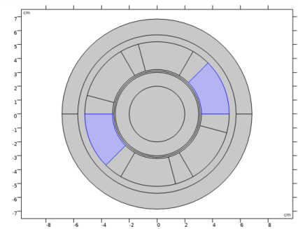
In the Model Builder window, expand the Coil, Phase B node, then click Reversed Current Direction 1.
2
In the Settings window for Reversed Current Direction, locate the Domain Selection section.
3
Click  Clear Selection.
4
Coil, Phase B
Specify the second coil current with a 120° phase shift with respect to the first. In frequency domain, this corresponds to a multiplication by a complex phase factor.
1
In the Model Builder window, click Coil, Phase B.
2
In the Settings window for Coil, locate the Coil section.
3
In the Icoil text field, type coil_wire_current*exp(j*2*pi/3).
Coil, Phase C
1
Right-click Coil, Phase B and choose Duplicate.
2
In the Settings window for Coil, type Coil, Phase C in the Label text field.
3
Locate the Domain Selection section. Click  Clear Selection.
4
Specify the third coil current with a -120° phase shift.
5
Locate the Coil section. In the Icoil text field, type coil_wire_current*exp(-j*2*pi/3).
Reversed Current Direction 1
1
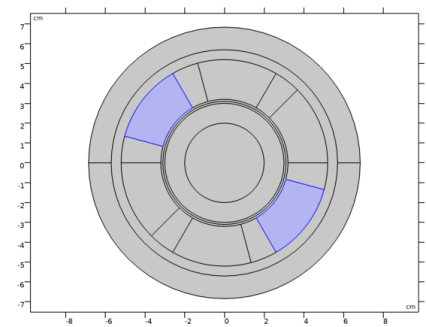
In the Model Builder window, expand the Coil, Phase C node, then click Reversed Current Direction 1.
2
In the Settings window for Reversed Current Direction, locate the Domain Selection section.
3
Click  Clear Selection.
4
Velocity (Lorentz Term) 1
1
In the Physics toolbar, click  Domains and choose Velocity (Lorentz Term).
2
3
In the Settings window for Velocity (Lorentz Term), locate the Coordinate System Selection section.
4
From the Coordinate system list, choose Cylindrical System 2 (sys2).
5
Locate the Velocity (Lorentz Term) section. Specify the v vector as
Here, Omega is the model parameter corresponding to the angular velocity, while sys2.r is the radial coordinate in the cylindrical coordinate system (with tag sys2).
Force Calculation 1
1
In the Physics toolbar, click  Domains and choose Force Calculation.
2
Mesh 1
Create an appropriate mesh for the model. The mesh must be fine enough at the surface of the rotating conductor to resolve the skin depth even with the highest slip. For this particular model, this is verified already with the default mesh.
1
In the Model Builder window, under Component 1 (comp1) right-click Mesh 1 and choose Build All.
Now, set up the study, using a parametric sweep for the rotational speed.
2
Right-click Component 1 (comp1)>Mesh 1 and choose Build Selected.
Study 1
Parametric Sweep
1
In the Study toolbar, click  Parametric Sweep.
2
In the Settings window for Parametric Sweep, locate the Study Settings section.
3
4
Step 1: Frequency Domain
1
In the Model Builder window, click Step 1: Frequency Domain.
2
In the Settings window for Frequency Domain, locate the Study Settings section.
3
In the Frequencies text field, type f0.
4
In the Study toolbar, click  Compute.
Results
Magnetic Flux Density Norm (mf)
After the solution has been computed, the default surface plot will be shown. Default plot visualize the magnetic flux density lines by means of a contour plot. This setting will be added explicitly in the after the second study.
1
In the Magnetic Flux Density Norm (mf) toolbar, click  Plot.
Create an additional plot for the current density induced in the rotor.
Current Density
1
In the Home toolbar, click  Add Plot Group and choose 2D Plot Group.
Specify a custom title for the plot. Using the Allow evaluation of expressions functionality, it is possible to include values (such as the rotational velocity Omega) in the title.
2
In the Settings window for 2D Plot Group, type Current Density in the Label text field.
3
Click to expand the Title section. From the Title type list, choose Manual.
4
Select the Allow evaluation of expressions check box.
5
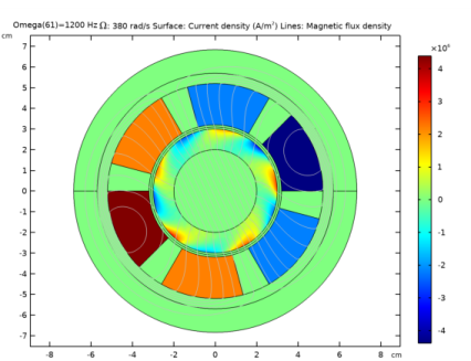
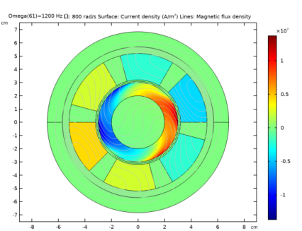
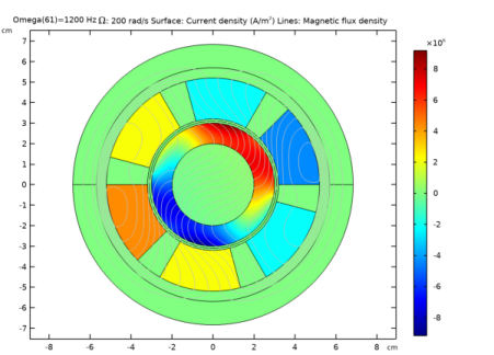
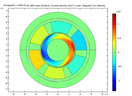
In the Title text area, type \OMEGA: eval(Omega) rad/s Surface: Current density (A/m<sup>2</sup>) Lines: Magnetic flux density.
Surface 1
1
Right-click Current Density and choose Surface.
2
In the Settings window for Surface, click Replace Expression in the upper-right corner of the Expression section. From the menu, choose Component 1 (comp1)>Magnetic Fields>Currents and charge>Current density - A/m²>mf.Jz - Current density, z component.
Contour 1
1
In the Model Builder window, right-click Current Density and choose Contour.
2
In the Settings window for Contour, click Replace Expression in the upper-right corner of the Expression section. From the menu, choose Component 1 (comp1)>Magnetic Fields>Magnetic>Magnetic vector potential - Wb/m>mf.Az - Magnetic vector potential, z component.
3
Locate the Coloring and Style section. From the Coloring list, choose Uniform.
4
From the Color list, choose Gray.
5
Clear the Color legend check box.
Current Density
1
In the Model Builder window, click Current Density.
2
In the Settings window for 2D Plot Group, locate the Data section.
3
From the Parameter value (Omega (Hz)) list, choose 200.
4
In the Current Density toolbar, click  Plot.
The plot shows how the field is affected by the rotor rotating more slowly than the field.
5
From the Parameter value (Omega (Hz)) list, choose 380.
6
In the Current Density toolbar, click  Plot.
At a speed close to the synchronous speed (377 rad/s) the field lines are not deformed and the induced current densities are at a minimum.
7
From the Parameter value (Omega (Hz)) list, choose 800.
8
In the Current Density toolbar, click  Plot.
The field applies a braking effect on the fast-spinning rotor.
Import the reference analytic data and compare it to the computed solution.
Reference Data
1
In the Results toolbar, click  Table.
2
In the Settings window for Table, type Reference Data in the Label text field.
3
Locate the Data section. Click Import.
4
Torque
1
In the Results toolbar, click  1D Plot Group.
2
In the Settings window for 1D Plot Group, type Torque in the Label text field.
3
Click to expand the Title section. From the Title type list, choose Manual.
4
In the Title text area, type Torque (N*m).
5
Locate the Plot Settings section. Select the x-axis label check box.
6
In the associated text field, type Angular Velocity (rad/s).
Global 1
1
Right-click Torque and choose Global.
2
In the Settings window for Global, click Replace Expression in the upper-right corner of the y-Axis Data section. From the menu, choose Component 1 (comp1)>Magnetic Fields>Mechanical>Torque - N·m>mf.Tz_0 - Torque, z component.
3
Click to expand the Legends section. From the Legends list, choose Manual.
4
In the table, type Computed in the first row.
Table Graph 1
1
In the Model Builder window, right-click Torque and choose Table Graph.
2
In the Settings window for Table Graph, locate the Data section.
3
From the Plot columns list, choose Manual.
4
In the Columns list, select Torque (N*m).
5
Locate the Coloring and Style section. Find the Line style subsection. From the Line list, choose None.
6
Find the Line markers subsection. From the Marker list, choose Cycle.
7
From the Positioning list, choose In data points.
8
Click to expand the Legends section. Select the Show legends check box.
9
From the Legends list, choose Manual.
10
In the table, type Reference in the first row.
11
In the Torque toolbar, click  Plot.
Coil Voltage
1
Right-click Torque and choose Duplicate.
2
In the Settings window for 1D Plot Group, type Coil Voltage in the Label text field.
3
Locate the Title section. In the Title text area, type Coil Voltage per Turn (V, RMS).
Global 1
1
In the Model Builder window, expand the Coil Voltage node, then click Global 1.
2
In the Settings window for Global, locate the y-Axis Data section.
3
Table Graph 1
1
In the Model Builder window, click Table Graph 1.
2
In the Settings window for Table Graph, locate the Data section.
3
In the Columns list, select Vin/turn (V).
4
In the Coil Voltage toolbar, click  Plot.
Rotor Losses
1
In the Model Builder window, right-click Coil Voltage and choose Duplicate.
2
In the Settings window for 1D Plot Group, type Rotor Losses in the Label text field.
3
Locate the Title section. In the Title text area, type Rotor Losses (W).
Global 1
1
In the Model Builder window, expand the Rotor Losses node, then click Global 1.
2
In the Settings window for Global, locate the y-Axis Data section.
3
Table Graph 1
1
In the Model Builder window, click Table Graph 1.
2
In the Settings window for Table Graph, locate the Data section.
3
In the Columns list, select Rotor_Loss (W).
4
In the Rotor Losses toolbar, click  Plot.
Steel Losses
1
In the Model Builder window, right-click Rotor Losses and choose Duplicate.
2
In the Settings window for 1D Plot Group, type Steel Losses in the Label text field.
3
Locate the Title section. In the Title text area, type Steel Losses (W).
Global 1
1
In the Model Builder window, expand the Steel Losses node, then click Global 1.
2
In the Settings window for Global, locate the y-Axis Data section.
3
Table Graph 1
1
In the Model Builder window, click Table Graph 1.
2
In the Settings window for Table Graph, locate the Data section.
3
In the Columns list, select Steel_Loss (W).
4
In the Steel Losses toolbar, click  Plot.
Current Density
Click the  Zoom Extents button in the Graphics toolbar.
Finally, to appreciate the dynamics of the rotating field, create an animation of the time-harmonic solution.
Animation 1
1
In the Results toolbar, click  Animation and choose Player.
2
In the Settings window for Animation, locate the Animation Editing section.
3
From the Sequence type list, choose Dynamic data extension.
4
Locate the Playing section. From the Repeat list, choose Forever.
5
In the Graphics toolbar, use the Play and Stop buttons to control the animation.