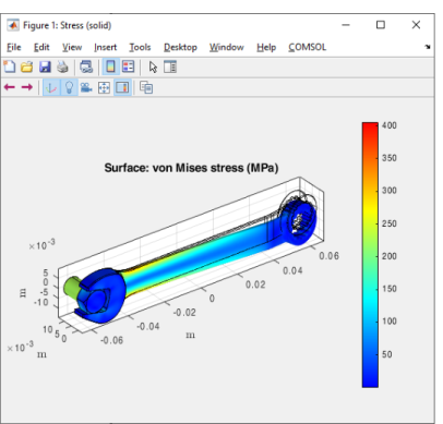
Displaying The Results
There are different commands available to Display Plot Groups, Extract Plot Data, Plot External Data, and to Add Data Plot to Model. A practical example of this is included in Example: Plot mpheval Data.
Display Plot Groups
Use the command mphplot to display a plot group available from the model
mphplot(model)
The figure contains a toolbar that allows the user to control the use of views, lights, and camera settings set in the model. The COMSOL menu list the plot group available, as well as geometry and mesh plot.
You can specify the plotgroup to display at the command line. For example, to display the plot group <pgtag> enter:
mphplot(model, <pgtag>)
mphplot does not support image features, Material Appearance subfeatures, and clipping views.
This renders the graphics in a MATLAB figure window. In addition you can plot results in a COMSOL Multiphysics Graphics window if you start COMSOL with MATLAB using a graphics COMSOL Multiphysics Server. To do this for a plot group <pgtag> enter:
mphplot(model, <pgtag>, 'server', 'on')
See the section Starting COMSOL Multiphysics with MATLAB using the Graphics Server in the COMSOL Multiphysics Installation Guide.
Another way to plot in a COMSOL Graphics window is to use the run method:
model.result(<pgtag>).run
The default settings for plotting in a MATLAB figure do not display the color legend. To include the color legend in a figure, use the property rangenum:
mphplot(model, <pgtag>, 'rangenum', <idx>)
where the integer <idx> identifies the plot for which the color legend should be displayed.
Extract Plot Data
In some situation it can be useful to extract data from a plot, for example, if you need to manually edit the plot as it is allowed in MATLAB. To get a cell array, pd, which contains the data for each plot feature available in the plot group <pgtag> enter:
pd = mphplot(model, <pgtag>)
The data fields contained in pd returned by mphplot are subject to change. The most important fields are:
p, the coordinates for each point that are used for creating lines or triangles.
n, the normals in each point for the surfaces. These are not always available.
t, contains the indices to columns in p of a simplex mesh, each column in t representing a simplex.
d, the data values for each point.
rgb, the color values (red, green and blue) entities at each point.
If you don’t want to generate a figure when extracting the plot data structure, set the property createplot to off as in the command below:
pd = mphplot(model, <pgtag>, 'createplot','off')
This is useful for instance on machine without graphics display support.
Example: Examining the plot data
Reuse the first on-line example available for mphplot:
model = mphopen('model_tutorial_llmatlab');
std = model.study.create('std');
std.feature.create('stat','Stationary');
std.run;
model.result.dataset.create('mir', 'Mirror3D');
pg = model.result.create('pg', 'PlotGroup3D');
pg.set('data', 'mir');
surf1 = pg.feature.create('surf1', 'Surface');
surf1.set('colortable', 'Thermal');
mphplot(model,'pg')
surf2 = pg.feature.create('surf2', 'Surface');
surf2.set('data', 'dset1').set('expr', 'ht.tfluxMag');
Now plot the result and extract the associated plot data structure:
pd = mphplot(model,'pg');
pd is a cell array containing three plot data structure, the first one corresponds the outline of the geometry, the title, the legend and the color bar information (if any) in the figure. The second and the third plot data structures correspond to the plot defined by the features added to the plot group pg: surf1 and surf2 respectively.
To inspect the outline data of the geometry enter:
pd1 = pd{1}{1}
pd1 =
             p: [3×1310 single]
             t: [2×1048 int32]
           rgb: [3×1 double]
          type: 'line'
      plottype: 'PlotGroup3D'
           tag: 'pg'
preserveaspect: 'on'
         title: 'Surface: Temperature (K) Surface: Total heat ...'
    titlecolor: [3×1 double]
   legendcolor: [3×1 double]
To investigate the plot data information of the second surface plot feature (surf2) enter:
pd3 = pd{3}{1}
pd3 =
p: [3x4917 single]
n: [3x4917 single]
t: [3x8964 int32]
d: [4917x1 single]
colortable: 'Rainbow'
       cminmax: [0.3193 6.7120e+05]
rgb: [4917x3 single]
type: 'surface'
plottype: 'Surface'
tag: 'surf2'
Code for use with MATLAB®
model = mphopen('model_tutorial_llmatlab');
std = model.study.create('std');
std.feature.create('stat','Stationary');
std.run;
model.result.dataset.create('mir', 'Mirror3D');
pg = model.result.create('pg', 'PlotGroup3D');
pg.set('data', 'mir');
surf1 = pg.feature.create('surf1', 'Surface');
surf1.set('colortable', 'Thermal');
mphplot(model,'pg')
surf2 = pg.feature.create('surf2', 'Surface');
surf2.set('data', 'dset1').set('expr', 'ht.tfluxMag');
pd = mphplot(model,'pg');
 
Plot External Data
Using the function mphplot you can also plot data that is specified directly as an input argument. The supported data format is according to the structure provided by the functions mphplot, mpheval and mphmesh.This allows you to plot data that has first been extracted from the model. To plot the structure <data>, run the command:
mphplot(<data>)
If the data structure contains the value of several expressions, set the one to display in the plot with the index property:
mphplot(<data>, 'index', <idx>)
where <idx> is a positive integer that corresponds to the expression to plot.
mphplot supports only plotting of data structures that are of the type point, line or surface evaluations from mpheval.
Using the colortable option to select from several available color tables when visualizing data:
mphplot(<data>, 'colortable', colorname)
Obtain a list of alternatives for colorname from the on-line help by entering:
help colortable
To disable the mesh displayed together with the data results, set the property mesh to off as in this command:
mphplot(<data>, 'mesh', 'off')
Add Data Plot to Model
Use the command mphaddplotdata to create a plot group and incorporate the data to a COMSOL Model. To create a plot group in the model using the plotdata data and using the plottype type, enter the command:
mphaddplotdata(model, 'type', type, 'data', data)
where type is the type of plot, that can be 'arrow', 'line', 'surface', 'annotation', 'tube' or 'point'.
You can create a plottype using the plotdata in an existing plotgroup using the property plotgroup as in the command below:
mphaddplotdata(model, 'type', type, 'data', data,...
'plotgroup', <pgtag> )
If you want to remove all existing plottype in the plotgroup enter:
mphaddplotdata(model, 'type', type, 'data', data,...
'plotgroup', <pgtag> , 'clearplot', 'on')
Example: Plot mpheval Data
This example extracts COMSOL data at the MATLAB prompt, modifies it and plots the data in a MATLAB figure.
First load the Busbar model from the COMSOL Multiphysics Applications Libraries. Enter:
model = mphopen('busbar');
To extract the temperature and the electric potential field, use the command mpheval:
dat = mpheval(model,{'T','V'},'selection',1);
To display the temperature field, using the thermal color table:
mphplot(dat,'index',1,'colortable','thermal');
Do a simple scaling of the electric potential then plot it using the default color table:
dat.d2 = dat.d2*1e-3;
Plot the newly evaluated data without the mesh:
mphplot(dat, 'index', 2, 'rangenum', 2, 'mesh', 'off');
To emphasize the geometry use the function mphgeom to display line plot on the same figure:
hold on;
mphgeom(model, 'geom1', 'facemode', 'off')
Code for use with MATLAB®
model = mphopen('busbar');
dat = mpheval(model,{'T','V'},'selection',1);
mphplot(dat,'index',1,'colortable','thermal');
dat.d2 = dat.d2*1e-3;
mphplot(dat, 'index', 2, 'rangenum', 2, 'mesh', 'off');
hold on;
mphgeom(model, 'geom1', 'facemode', 'off')