Use state-space export to create a linearized state-space model corresponding to a COMSOL Multiphysics model. You can export the matrices of the state-space form directly to the MATLAB® workspace with the command mphstate.

This section includes information about The State-Space System, how to Extract State-Space Matrices and Set Linearization Points and has an Extracting State-Space Matrices.

where x is the state variable vector.

If the components of the mass matrix MC are small, it is possible to approximate the dynamic state-space model with a static model, where :

Let Null be the PDE constraint null-space matrix and ud a particular solution fulfilling the constraints. The solution vector U for the PDE problem can then be written

where u0 is the linearization point, which is the solution stored in the sequence once the state-space export feature is run.

The input parameters should contain all parameters that are of interest as input to the model. Moreover if you have any settings in model that are connected to the degrees of freedom, like a constraint condition or a spring condition. These have to be declared as input in your state-space system. When solving the state-space system in MATLAB, subtract to these inputs the initial value of the corresponding DOF, as it is done in the example Extracting State-Space Matrices.

The function mphstate requires that the input variables, output variables, and the list of the matrices to extract in the MATLAB workspace are all defined:

where <soltag> is the solver node tag used to assemble the system matrices listed in the cell array out, and <input> and <output> are cell arrays containing the list of the input and output variables, respectively.

The output data str returned by mphstate is a MATLAB structure and the fields correspond to the assembled system matrices.

The system matrices that can be extracted with mphstate are listed in the table:

To extract sparse matrices set the property sparse to on:

To keep the state-space feature node, set the property keepfeature to on:

mphstate uses linearization points to assemble the state-space matrices. The default linearization point is the current solution provided by the solver node, to which the state-space feature node is associated. If there is no solver associated to the solver configuration, a null solution vector is used as a linearization point.

You can manually select the linearization point to use. Use the initmethod property to select a linearization point:

where method corresponds to the type of linearization point — the initial value expression ('init') or a solution ('sol').

To set the solution to use for the linearization point, use the property initsol:

where <initsoltag> is the solver tag to use for a linearization point. You can also set the initsol property to 'zero', which corresponds to using a null solution vector as a linearization point. The default is the current solver node where the assemble node is associated.

For continuation, time-dependent, or eigenvalue analyses you can set which solution number to use as a linearization point. Use the solnum property:

where <solnum> is an integer value corresponding to the solution number. The default value is the last solution number available with the current solver configuration.

State space models can be defined using the ss or sparss function. The sparss function can be used if the state space matrices are sparse. The system can be simulated using the lsim function. In order to create a reduced order system using MATLAB we will use the balred function. This function only accepts the use of full matrices. Hence, the function ss is used for defining the state space system in MATLAB. Note that calling the function ss with argument matrices that are sparse result in a set of warnings. These warnings can be ignored.

The code below show how to use the Control System Toolbox to solve a dynamic system from the A, B, C, and D matrices obtained using mphstate:

where <input> is the input vector of the state space system, <tspan> the time step list.

One may obtain a reduced order model using the balred function.

where <order> is the desired order reduction, and <tfinal> the simulation end time.

In this section you will find an example that illustrate how to use the mphstate function to extract the state-space matrices.

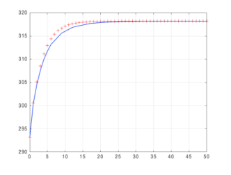
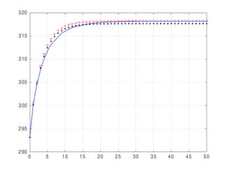
This is the same problem solved as in Extracting Reduced Order State-Space Matrices so you can compare the solution, and computational performance when solving the problem with reduced order model state space system matrices.

Extract the state-space system matrices Mc, MA, MB, C, and D, of the model with power, Temp, and Text as input and the probe evaluation comp1.ppb1 as output:

Compare the solution computed with the system and the one computed with COMSOL Multiphysics (see Figure 4-1):

For some types of control system design the use of the matrices A, B, C, and D are commonly used. Note that you need to keep the size of the matrices lower as you are not using a mass matrix. Hence, you need to change the size of mesh in order to reduce the number of degrees of freedom of the assembled system:

Extract the state-space system matrices A, B, C, and D, of the model with power, Temp, and Text as input and the probe evaluation comp1.ppb1 as output:

Compare the solution computed with the previous system (see Figure 4-2):