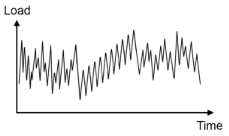
Fatigue damage caused by a random load history or a variable load (see Figure 3-15) is not as easily quantified as damage from a constant load cycle. Correct simulation of the fatigue process plays a key role to predict the life of the structure. The nature of the service load history needs to be determined and the accumulated damage must be defined.

In the Cumulative Damage evaluation, the load is first processed with the cycle counting method, rainflow counting (Ref. 2), and followed by the damage estimation according to the Palmgren-Miner linear damage model (Ref. 3).

The Rainflow counting method counts load cycles and transfers it into a stress distribution of the applied load history. Before this can be done, the stress tensor needs to be converted into an equivalent scalar stress. This choice is done in the specification of the Stress settings in the Cycle Counting Parameters section. The following stress definitions can be evaluated:

In the expressions in Table 3-6, σ is the stress measure used in the Rainflow cycle counting method, σ1 is the largest principal stress, σ3 is the smallest principal stress, σvM is the von Mises equivalent stress, and σh is the hydrostatic (or mean) stress.

The Rainflow counting method reduces the stress history into a stress distribution that consists of a discrete number of bins, where each bin is characterized by an amplitude stress, σa, and a mean stress, σm, and holds the counted number of cycles having approximately these values. Other parameters can also be used to define a bin. These are maximum stress, minimum stress, maximum tensile stress, or R-value. In Figure 3-16 an example of a dataset is shown where the load history has been reduced to 16 bins. In the bin σa = 70 MPa and σm = 30 MPa, 67 load cycles are found. This means that in the original load response 67 cycles are present in the range 65 MPa<σa <75 MPa and 25 MPa<σm<35 MPa.

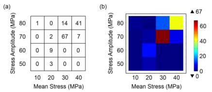
The rainflow counted cycles of all bins are collected in the variable ftg.csc (counted stress cycles). This variable can be visualized with the Matrix Histogram, see Figure 3-16.

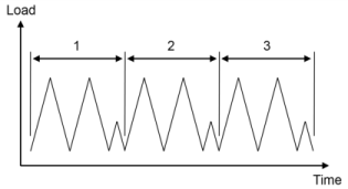
where ni is the number of cycles in bin i, Ni is the maximum number of cycles until fatigue occurs for bin i, q is the number of bins, and m is number of repeated cycle blocks in the load history, see Figure 3-17. Usually a fatigue usage factor of 1 or larger means that the component fails due to fatigue.

If the cycles in the bins describe the entire load history, the stress cycle is not repeated and thus m = 1.

The limiting stress as a function of the number of cycles until failure is obtained from the S-N curve, also called the Wöhler curve, see Figure 3-18. For different R-values (R), different material responses can be expected.

It is recommended that the S-N curve is defined using an Interpolation function of Grid type, or with an Analytical function. Other function types can also be used. It is important that the arguments of the function are ordered with R-value as the first argument and number of cycles as the second argument.

The evaluation of the S-N curve in the Cumulative Damage node is based on the following relations:

The cumulative damage depends on the combination of stress levels and the number of counted cycles (see Equation 3-3). Each bin contributes to the fatigue usage factor with

where index i denotes the bin counter. The contribution to fus by all bins is collected in the relative usage factor ftg.rus. The sum of all individual components of the relative usage factor is 1.

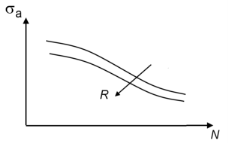
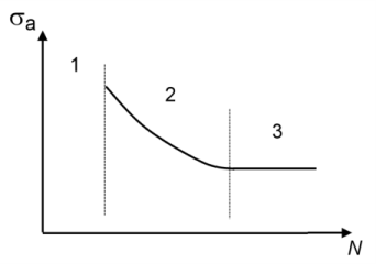
The S-N curve can be divided into three regions, shown in Figure 3-19. At high stresses, region 1, the fatigue life cannot be predicted since other mechanisms than the stress amplitude control fatigue. In this regime low-cycle fatigue and static failure can be expected. At intermediate stresses, region 2, the fatigue life is well defined and follows the S-N curve. At stresses below the endurance limit, the life is infinite and fatigue will not occur.

The results calculated in the fatigue analysis depend on the location at the S-N curve where a stress cycle is encountered. Sometimes, it is not possible to determine a lifetime (number of allowed cycles) for a certain stress bin. Table 3-7 summarizes the results which can occur. For certain cases, there is a difference depending on whether a single point is evaluated or multiple points are evaluated. Generally, when stresses are within the finite life region all results are well defined and computed. When a single point is evaluated the counted stress cycles can always be computed but the computation of remaining results depends on the life region were stresses are encountered.

In Table 3-7, “Undefined” means that results are undefined and cannot be computed, “Defined” means that results are well defined and are computed, and “Zero” means that results are stored as zero. In an analysis where results are available in some regions, the fatigue usage factor is always displayed. In regions where undefined life is encountered, no results are computed. In case of a 2D plot, no color is shown in such areas as demonstrated in Figure 3-20.

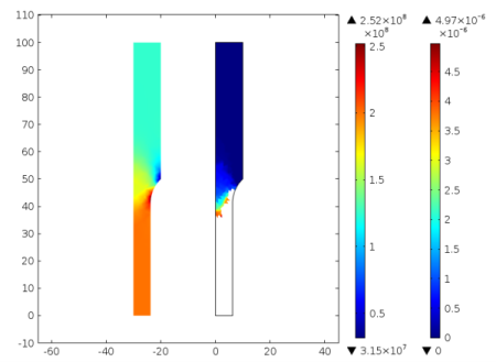
The example shown in Figure 3-20 is based on an S-N curve with top stress of 200 MPa and endurance limit at 125 MPa. This means that when stresses are above 200 MPa, a fatigue life cannot be predicted, and when stresses are below 125 MPa an infinite life is expected. In the example, stresses below 125 MPa are experienced in the thick top part of the specimen, and as a result a zero usage factor is calculated in this region. Stresses above 200 MPa are experienced in the thin bottom part of the specimen. As the fatigue usage factor cannot be defined in this part, no results are calculated in this region, as indicated by the missing color contours in the right picture. If a computed stress amplitude exceeds the highest stress amplitude in the S-N curve, a warning stating that fatigue could not be evaluated is displayed.

The influence of the total load history is described in a number of modeling steps. Refer to Figure 3-23 to see an example of the steps as explained next.

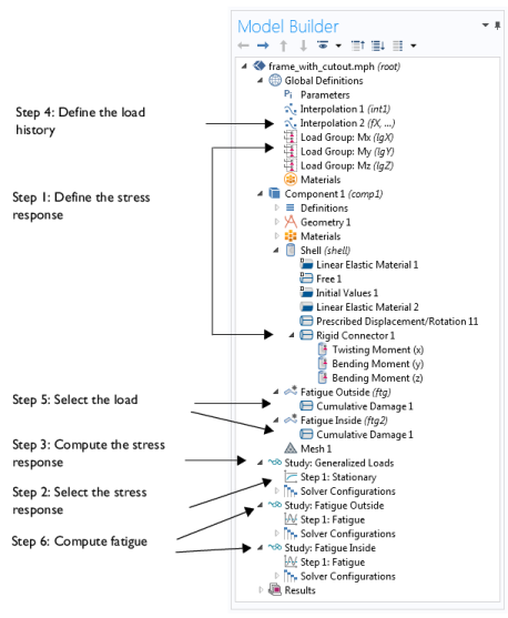
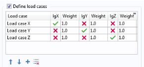
Start by computing σijk. Then define generalized unit loads as Load Groups (step 1) and set up the solution in the Define load cases option of the Study Extensions section in the preceding stress/strain Study (step 2), see Figure 3-21.

When the study is computed (step 3), σijk is calculated and acts as a multiplier to the time history of the generalized loads, fk.

Provide load histories using functions under Global Definitions (step 4) and further specify the functions with the name in the Generalized load history parameter of the Generalized Load Definition section in the Cumulative Damage node (step 5) (Figure 3-22).

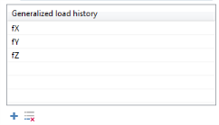
The order of generalized unit loads in the stress/strain Study must correspond to the order of load histories specified in the Generalized load history parameter; compare Figure 3-21 with Figure 3-22. Finally, calculate the fatigue usage factor by solving the fatigue study (step 6). All steps are schematically shown in Figure 3-23.

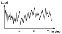
The load history evaluated by the cycle counting method is limited by the Initial step si and Final step sf parameters (see Figure 3-24). This makes it possible to evaluate the influence of parts of the load history on the cumulative damage, with no change of the load history function. See Figure 3-24.