Theory for FSDT Laminated Shell
The theory of laminated shells is discussed in this section. The Layered Linear Elastic Material node in the Shell interface allows the modeling of laminated shells, also popularly known as composite laminates, having different orthotropic properties per layer. The first order shear deformation theory (FSDT) is used to find homogenized equivalent material properties of a composite laminate.
The Layered Linear Elastic Material is only available in the Composite Materials Module.
The Layered Linear Elastic Material is only available in 3D and not in 2D axisymmetry.
Several topics are discussed in this section:
About Composite Laminates
A layered shell, also known as a composite laminate, is a thin-walled structure in 3D having many layers of different orthotropic (or optionally isotropic/anisotropic) material stacked on top of each other.
A layered shell can be active either on free surfaces embedded in 3D, or on the boundary of a solid object in 3D. In the latter case, it can be used to model a reinforcement on the surface of a solid object. A simple form is assumed for the variation of the displacement through the thickness in order to develop a model for the deformation that is more similar to a 2D plane stress condition than to a full 3D state.
Figure 5-3: Geometry of a doubly curved composite laminate.
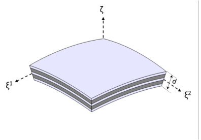
Figure 5-3 shows a doubly curved laminated shell with uniform total thickness, d. It is represented by orthogonal curvilinear coordinate system (ξ1, ξ2, ζ). The geometry representation of a layered shell is same as a single layer shell as discussed in the Geometry and Deformation section.
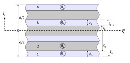
A typical stacking sequence of a composite laminate having n layers is shown in Figure 5-4. The thickness of each layer (dk), as well as the fiber direction in each layer (θk) with respect to the first principal direction (ξ1) of the laminate are indicated. A counterclockwise rotation of the fiber direction with respect to the ζ direction is considered as positive.
Figure 5-4: A typical stacking sequence of a composite laminate showing thickness and fiber orientation in each layer.
Equivalent Single Layer (ESL) Theory
Composite laminates are formed by stacking layers of different materials or having different fiber orientations. In general, composite laminates have a planar dimension that is orders of magnitude larger than the thickness. They are often used in the applications requiring membrane and bending strengths. Therefore, composite laminates can often be modeled using a shell element based on an equivalent single layer (ESL) theory.
In ESL theory, a heterogeneous laminated shell is converted into a statically equivalent single layer shell by reducing the 3D continuum problem to a 2D shell problem. In addition to their simplicity and low computational cost, ESL theory provides sufficiently accurate description of global response for a thin to moderately thick laminates, for example gross deflections in a laminate, critical buckling loads, and eigenfrequencies with corresponding mode shapes.
Assumptions and Restrictions
Some of the general assumptions when using shell theory to model a thin solid structure are:
Some of the assumptions specific to ESL theory when used to model a composite laminate are:
Classification
The ESL theories can be classified into various groups based on the description of the transverse shear stresses.
Classical Laminate Plate Theory (CLPT)
 
The classical laminate plate theory is an extension of Kirchhoff or classical plate theory used for single layer thin shells. In this theory, transverse shear stresses are neglected and the deformation is entirely due to the bending and in-plane stretching.
First Order Shear Deformation Theory (FSDT)
 
The first order shear deformation theory is similar to the Mindlin-Reissner shell theory used for single layer thick shells. This theory extends the kinematics of CLPT by including the gross transverse shear deformation. The transverse shear strain is assumed to be constant with respect to the thickness coordinate. As the transverse shear strain has a constant value, this theory requires a shear correction factor.
Higher Order or Third Order Shear Deformation Theory (HSDT)
 
This theory is an extension of FSDT where the displacement field is approximated in such a way that the transverse shear strain varies quadratically with respect to the thickness coordinate. It makes the transverse shear stresses zero at the top and bottom surfaces of the laminate, thus eliminating the need of a shear correction factor.
First Order Shear Deformation Theory (FSDT)
In COMSOL Multiphysics, the first-order shear deformation theory (FSDT) is implemented to model composite laminates using an equivalent single layer approach. The element used for the shell interface is of Mindlin-Reissner type, which means that transverse shear deformations are accounted for. It can thus also be used for rather thick shells. It has an MITC (mixed interpolation of tensorial components) formulation.
FSDT differs from the single layer shell theory in the way through-thickness integrations are performed, constitutive equations are formed, and results are evaluated. In the following sections, these topics are discussed in detail.
Integration in a Laminate
All volume integrals over a shell element are split into a surface integration and a through-thickness integration. Both integrations are performed numerically. The surface geometry is used for surface integration, and an extra dimension geometry is used for the through-thickness integration. It is thus possible to enter data which depend on the thickness direction.
Unlike a single layer shell, where all material properties are evaluated at the reference surface, different material and fiber orientation can be specified in each layer of the composite laminate. Formally this can be written as:
For curved laminates, an area scale factor is also included since the layers have different surface area. This is independent of whether an offset is used or not, but the offset affects the scale factor. The definition of the area scale factor (ASF) for a composite laminate is similar to that of a single layer shell.
Lamina Constitutive Law
In classical laminate theory, a lamina is assumed to be in a plane stress state and all three transverse stress components (σxz, σyz, σzz) are assumed to be zero. In terms of strains, the transverse shear strain components (εxz, εyz) are zero while the transverse normal strain (εzz) is nonzero but not part of the formulation.
FSDT extends the classical laminate theory and allows nonzero transverse shear strain components.
In-plane Constitutive Equations (Membrane and Bending Equations)
The linear constitutive relation for orthotropic lamina k in a composite laminate, can be written as:
where
σij are the stress components in the principal material directions of a lamina
εij are the strain components in the principal material directions of a lamina
Qij are the elasticity matrix components in the principal material directions of a lamina
For an orthotropic lamina, the elasticity matrix components (Qij) can be defined in terms of the material constants ():
A general composite laminate is made of several orthotropic layers, having principal material directions with different orientations with respect to the laminate coordinates (ξ1, ξ2, ζ) as shown in Figure 5-3. The constitutive equations for a lamina can be transformed from its material coordinate system to the laminate coordinate system, giving:
where
 σij are the stress components in the laminate coordinate system
εij are the strain components in the laminate coordinate system
Qij are the elasticity matrix components in the laminate coordinate system
The transformed in-plane elasticity matrix is defined as:
The principal material direction (or fiber direction) in each lamina makes an angle (θ) with the first in-plane direction (ξ1) of the laminate coordinate system. Hence the transformation matrix can be defined as:
where c = cos θ and s = sin θ.
Out-of-plane Constitutive Equations (Shear Equations)
The linear constitutive relation for the transverse shear in a lamina k can be written as:
where
 σij are the transverse shear stress components in the principal material directions of a lamina
εij are the transverse shear strain components in the principal material directions of a lamina
Qij are the elasticity matrix components in the principal material directions of a lamina
For an orthotropic lamina, the elasticity matrix components (Qij) can be defined in terms of the two shear moduli ():
The constitutive equations of a lamina can be transformed from its material coordinate system to the laminate coordinate system and can be written as:
where
 σij are the transverse shear stress components in the laminate coordinate system
εij are the transverse shear strain components in the laminate coordinate system
Qij are the elasticity matrix components in the laminate coordinate system
The transformed out-of-plane elasticity matrix is defined as:
where the transformation matrix is defined as:
Laminate Constitutive Law
The laminate constitutive law relates the resultant membrane forces, bending moments, and transverse shear forces to the membrane strains, bending strains, and transverse shear strains.
Figure 5-5: An equivalent layer of a composite laminate having n layers. The resultant membrane forces (), bending moments (), and transverse shear forces () are shown.
The resultant membrane forces, bending moments, and transverse shear forces in a composite laminate are computed as:
where
For shallow shells, the following approximation can be used:
This leads to
Hence the expressions for the resultant membrane force, bending moment, and transverse shear force reduce to the following:
This formulation, with its assumption of a moderate curvature, is the one used in the Shell interface.
The stress components can be written in terms of elasticity matrix components and strain components by using the lamina constitutive law. This establishes the relation between resultant forces and the midplane strains as given below:
The resultant force and moment expressions can be further rewritten as:
where
The extensional, bending, and coupling stiffnesses are defined as:
The in-plane laminate constitutive law, relating resultant forces and midplane strains, can also be written in matrix form as:
The midplane strains can be written using resultant forces and flexibility matrices as:
where
The stiffness and flexibility matrices are available for output, using for example Derived Values->Point Matrix Evaluation. The following matrix variables are defined:
Shear Correction Factor Computation
The transverse shear strains and stresses computed from the FSDT theory are averaged values. For this reason, they need shear correction factors in order to give correct strain energy contributions.
In order to compute the shear correction factor, the following assumptions are taken:
These assumptions are only satisfied exactly for a laminate with isotropic layers. For a laminate with orthotropic layers, the first assumption does not hold exactly but is approximately satisfied. The second assumption only holds for a cross-ply laminate having 0 and 90 degree layers.
For a laminate with isotropic layers, transverse shear stress are zero at free surfaces and they are continuous at interfaces between two layers. The through-thickness profile matches the 3D elasticity solution very closely. For a laminate with orthotropic layers, the zero shear stress condition is achieved at free surfaces of a laminate, while shear stress continuity at the interfaces is not guaranteed.
Based on the first assumption, the through-thickness derivative of a transverse strain component can be defined as:
Integrating the above equation in through-thickness direction, the transverse shear strain in each layer can be written as:
where
The transverse shear stress for each layer can be written as:
For n number of layers in a laminate, there are n+2 variables (unknowns) and thus n+2 equations are needed to solve them. The first n+1 equations are the form of shear stress continuity can be written as:
Here, the subscript indicates the layer index, and the superscript indicates the interface position (top or bottom) of a particular layer.
The missing equation can be expressed in the form of the average shear stress:
Using this set of equations, it is possible to solve for the correct distribution of shear stresses and strains. In order to compute the shear correction factor for the strain energy contribution, an additional equation is needed. It can be obtained through an energy equivalence approach between 3D elasticity and FSDT formulations.
The transverse shear strain energy based on the 3D elasticity theory is written as:
where the shear strain distribution is defined as:
The transverse shear strain energy, corresponding to (ε13), based on FSDT theory is written as:
The shear correction factor can be obtained by equating the two energy equations:
Similarly the shear correction factor corresponding to (ε23) is:
Results Evaluation in a Laminate
For visualization and results evaluation, predefined variables include all nonzero stress and strain tensor components, principal stresses and principal strains, in-plane and out-of-plane forces, moments, and von Mises and Tresca equivalent stresses.
Stresses and strains are available in the global coordinate system, laminate coordinate system, as well as in the layer local coordinate system.
Layered Material Slice Plot
It is possible to evaluate the stress and strain tensor components and equivalent stresses in each layer of a laminate using Layered Material Slice plot.
The through-thickness location can be set to evaluate a quantity in the middle of a layer, at an interface between two layers, top or bottom of a laminate etc. The top, bottom, and the middle of a laminate can be defined as:
Bottom of a laminate: 1 (relative) and 0 (physical)
Middle of a laminate: 0 (relative) and d/2 (physical)
Top of a laminate: +1 (relative) and d (physical)
The default value of though thickness location is given in the Default through-thickness result location section of the Layered Shell interface.
Through Thickness Plot
The through-thickness variation of a quantity at one or more locations on the reference surface can be plotted using a Through Thickness plot. In this plot, the reference surface locations can be specified through following ways:
Layered Material Data Set
The Layered Material data set allows the display of results in 3D solid even though the equations are solved on a 2D surface.
Using this data set, results can either be visualized on a 3D object or on slices created in the through-thickness direction of a 3D object. The following options are available in the data set to create slices in the through-thickness direction:
Sometimes, when a laminate is very thin, it becomes difficult to distinguish between a surface or a solid object. In such cases it is possible to scale the through-thickness direction in the data set for better visualization.