General Theory for the Shell and Plate Interfaces
Several topics are discussed in this section:
Geometry and Deformation
Let r be the undeformed shell midsurface position, ξi be element local (possibly nonorthogonal) coordinates with origin in the shell midsurface, and n be the normal to the undeformed midsurface. The thickness of the shell is d, which can vary over the element. The local coordinates ξ1 and ξ2 follow the midsurface, and ξ3 is the coordinate in the normal direction. The normal coordinate has a value of d/2 on the bottom side of the element, and +d/2 on the top side.
The position of the deformed midsurface is r + u, and the normal after deformation is n + a. To keep the normal a unit vector requires that
(5-1)
In a geometrically linear analysis Equation 5-1 is replaced by the simpler linearized form
since the formulation in that case assumes that
The vectors r, u, n, and a are interpolated by the nth-order Lagrange basis functions. The basic assumption is that the position of a point within the shell after deformation has a linear dependence of the thickness coordinate, and thus is
The superscripts indicate contravariant indices, while subscripts indicate covariant indices.
In axial symmetry, the local curvilinear coordinates have a special interpretation: ξ1 is the arc-length along the line on which the shell is modeled, and ξ2 is a circumferential coordinate given by ξ2 = RΘ.
Strains
The in-plane Green-Lagrange strain in the local covariant components can then be written as
The indices α and β range from 1 to 2. The transverse shear strains in local covariant components are
The constitutive relation for the shell elements is a plane stress assumption, as is customary in shell theory. The strain component in the normal direction ε33 is thus irrelevant. The different parts of the strain tensors above can be written out as
In a geometrically linear analysis, the nonlinear terms (products between u, a, and their derivatives) disappear. In all study types, the contributions from the parts καβ and ωα are ignored. They are small unless the element has an extremely high ratio between thickness and radius of curvature, in which case the errors from using shell theory are large anyway.
Note that ζα here is a strain component, not to be confused with the local coordinate in the normal direction or offset.
Offset
It is possible to model a shell with a midsurface that is not located at the meshed surface but at a certain offset from it. The offset is assumed to occur along the normal of the shell surface. In this case,
where rR is the position of the meshed reference surface and ζo is the offset distance.
Since all geometric derivatives are computed at the mesh on the reference surface, the following type of expressions are used when evaluating the strains:
The degrees of freedom are located on the reference surface.
All loads and boundary conditions are assumed to be applied at the midsurface, so a force acting in the plane of the shell does not cause any bending action if there is an offset.
The numerical integration of the element is performed over the reference surface. If the shell is curved, the area of the actual midsurface and the reference surface differ. This is compensated for by multiplying the weak expressions with an area scale factor, defined as
Any expressions depending on the coordinates are evaluated on the shell reference surface.
For conditions applied to edges, a similar length scale factor is required. It is defined as
where t is the tangent to the edge. For an internal edge, it is possible that there is a discontinuity in thickness or offset. In such a case, the line scale factor will be an average. Edge conditions in are not well defined in such situations because the position of the midsurface can be discontinuous. In practice, errors caused by such effects are small.
Rotation Representation
In a geometrically linear analysis, a rotation vector is defined as
In a geometrically nonlinear analysis, the rotation vector axis is defined by
while the amplitude of the rotation vector is computed as
This representation is unique only for rotations up to 180 degrees, but since the rotation vector representation is only an output convenience, it has no impact on the analysis.
The MITC Shell Formulation
The MITC formulation (Ref. 1) does not take the strain components directly from the shape functions of the element. Instead, meticulously selected interpolation functions are selected for the individual strain components. The values of the interpolated strains are then at selected points in the element tied to the value that would be computed from the shape functions. The interpolation functions and tying points are specific to each element shape and order.
Each contribution to the virtual work of the element is numerically integrated over the reference surface while the integration in the thickness direction is performed analytically. The computation of the strain energy from transverse shear deformations uses a correction factor of 5/6 to compensate for the difference between the assumed constant average shear strain and the true parabolic distribution.
Fold Lines
In regions where the discretized surface is smooth (which is always the case for plates), the normal of the shell surface is uniquely defined. When two or more shell elements meet at an angle, each element must however keep its own normal direction. It is thus not possible to have the same set of degrees of freedom for the displacement of the normal in such a point. This is automatically handled by the program. The automatic search for these fold lines compares the normals of all boundaries sharing an edge. If the angle between the normals is larger than a certain angle (with a default of 3 degrees) it is considered as a fold line. For a fold line, the assumption is that the angle between the shell normals remains constant. This gives
or
(5-2)
where the values or j and k range over the number of shells elements with different normals. The third term in Equation 5-2 is relevant only in a large deformation analysis because it is nonlinear. A special case occurs when two adjacent boundaries are parallel but their normal vectors have opposite directions. In this case the special constraint
is applied along their common edge.
Integration
All volume integrals over a shell element are split into a surface integral, which is performed numerically, and a thickness direction integral which is performed analytically. It is thus not possible to enter data which depend on the thickness direction. All material properties are evaluated at the reference surface. Formally this can be written as
All functions of ζ are assumed to be of the form ζn. Odd powers will integrate to zero, so typically the cross thickness integration will give factors d (for the case n = 0) and d3/12 (for the case n = 2). The thickness d can be a function of the position.
Initial Values and Prescribed Values
Because the normal vector displacements are quantities which are less intuitive than the more customary nodal rotations, it is possible to specify the prescribed values in terms of nodal rotations as well as in terms of the normal vector displacement. The representation by normal vector direction is insensitive to whether the analysis is geometrically nonlinear or not. The direction of the shell normal is prescribed in the deformed state, n0. The prescribed values for the actual degrees of freedom, a0, are internally computed as
If the rotation vector input is used, and the analysis is geometrically linear, then
where Ω0 is the vector of prescribed nodal rotations. This relation is fully defined only when all three components of Ω0 are given. It is also possible to prescribe only one or two of the components of Ω0, while leaving the remaining components free. Because it has no relevance to prescribe the rotation about the normal direction of the shell, it is only possible prescribe individual rotations in a shell local system. In this case, the result becomes one or two constraint relations between the components of a0. The directions are the edge local coordinate system where t1 is the tangent to the edge and t2 is perpendicular and inward from the edge, in the plane of the shell. These constraints are formulated as
Here Ω0i is the prescribed rotation around the axis ti.
In a geometrically nonlinear analysis, it is not possible to prescribe individual elements of the rotation vector. If only one or two components have been specified, the remaining components are set to zero. The actual degrees of freedom are then computed as
where R is a standard rotation matrix, representing the finite rotation about the given rotation vector.
Initial velocities are always given using an angular velocity vector ω as
Symmetry and Antisymmetry Boundary Conditions
It is possible to prescribe symmetry and antisymmetry boundary conditions. As a default, they are expressed in a shell local coordinate system. If applied to a boundary, the normal to the shell is assumed to be the normal to the symmetry or antisymmetry plane. The conditions are
for the symmetry case and
for the antisymmetry case. Here t1 and t2 are two perpendicular directions in the plane of the shell.
When applied to an edge, there is a local coordinate system where t1 is the tangent to the edge, and t2 is perpendicular and in the plane of the shell. The assumption is then that t2 is the normal to the symmetry or antisymmetry plane. The constraints are
for the symmetry case and
for the antisymmetry case.
When symmetry or antisymmetry conditions are specified in a general coordinate system with axis directions ei, i = 1, 2, 3 with e1 as the normal to the symmetry/antisymmetry plane the constraints are
or the symmetry case and
for the antisymmetry case. Using a general coordinate system sometimes leads to higher accuracy, since there is no element interpolation of the constraint directions involved.
Axisymmetric Models
In axisymmetric models, the only possible symmetry plane is the one having the Z-axis as normal. In this case, you can use the Symmetry Plane boundary condition. The imposed constraint is
External Loads
Contributions to the virtual work from the external load is of the form
where the forces (F) and moments (M) can be distributed over a boundary or an edge or concentrated in a point. The contribution from the normal vector displacement a is only included in a geometrically nonlinear analysis. Loads are always referred to the midsurface of the element. In the special case of a follower load, defined by its pressure p, the force intensity is
For a follower load, the change in midsurface area is not taken into account, in order to be consistent with the assumption that thickness changes are ignored.
Stress and Strain Calculations
The strains calculated in the element are, as described above, the covariant tensor components. They have little significance for the user, and are internally transformed to a Cartesian coordinate system. This system can be global or element local. The stresses are computed by applying the constitutive law to the thus computed strain tensor.
Each part of the covariant strain (γαβ, χαβ, ζα) is transformed separately. They correspond to membrane, bending, and shear action, respectively, and it is thus possible to separate the stresses from each of these actions. The membrane stress is defined as
where D is the plane stress constitutive matrix, Ni are the initial membrane forces, and γi the initial membrane strains. The influence of thermal strains is included through the midsurface temperature Tm, and the hygroscopic swelling through the midsurface moisture concentration, cm.The membrane stress can be considered as the stress at the midsurface, or as the average through the thickness.
The bending stress is defined as
where χi is the initial value of the bending part of the strain tensor (actually: the curvature), and Mi are the initial bending and twisting moments. ΔT is the temperature difference between the top and bottom surface of the shell, and Δcmo is the difference in moisture concentration between the top and bottom. The bending stress is the stress at the top surface of the shell if no membrane stress is present.
The average transverse shear stress is defined as
where G represent the transverse shear moduli, ζi is the initial average shear strain, and Qi are the initial transverse shear forces. The correction factor 5/6 ensures that the stresses are averaged so that they correspond to the ratio between shear force and thickness. The corresponding strains ζ and ζi are averaged in an energy sense.
The actual in-plane stress at a certain level in the element is then
where z is a parameter ranging from 1 (bottom surface) to +1 (top surface). The computation of the shear stress at a certain level in the element uses the following analytical parabolic stress distribution:
The shell section forces (membrane forces, bending moments, and shear forces) are computed from the stresses as
Local Coordinate Systems
Boundaries
Many quantities for a shell can best be interpreted in a local coordinate system aligned to the shell surface. Material data, initial stresses and stress results are always represented in this local coordinate system. You specify the orientation of the local directions in a Shell Local System node under the Linear Elastic Material.
The local system for stress output coincides with the orientations defined for the material input. Stresses are also available transformed to the global coordinate system.
If a Boundary System is selected, then the orientation of the shell local system is fully defined by the boundary system. When using a boundary system, it also possible to control the orientation of the shell normal by selecting the Reverse normal direction check box.
Other types of coordinate systems are not necessarily aligned with the shell surface. For such systems, the definition of the local shell surface coordinate system is as follows:
1. The local z direction ezl is the positive geometry normal of the shell surface.
2. The local x direction exl is the projection of the first direction in the material coordinate system (ex1) on the shell surface
This projection cannot be performed if ex1 is normal to the shell. In that case, the second axis ex2 of the material system instead defines exl using the same procedure. Thus, if
then
3. At last, the second in-plane direction is generated as
This procedure is followed irrespective of whether a global or a local coordinate system defines the directions.
Note the following:
For shells in the XY-plane, and for plates, the global and local directions coincide by default.
Local edge system
Many features, such as an edge load, allow input in an edge local coordinate system. The orthogonal local edge coordinate system directions xl, yl, and zl are defined so that:
The first direction (xl) is along the edge. This direction can be visualized by selecting the Show edge directions arrows check box in the View settings.
The third direction (zl) is the same as the shell normal direction. The shell normal direction can be visualized in the default plot named Undeformed geometry, or by adding a Coordinate System Surface plot and selecting the Shell, Local System.
The second direction (yl) is in the plane of the shell and orthogonal to the edge. It is formed by the cross product of zl and xl; yl = zl × xl.
When an edge is shared between two or more boundaries, the directions may not always be unique. It is then possible to use the control Face Defining the Local Orientations to select from which boundary the normal direction zl should be picked. The default is Use face with lowest number.
If the geometry selection contains several edges, the only available option is Use face with lowest number, since the list of adjacent boundaries would then be different for each edge. For each edge in the selection, the face with the lowest number attached to that edge is then used for the definition of the normal orientation.
Results Evaluation
For visualization and results evaluation, predefined variables include all nonzero stress and strain tensor components, principal stresses and principal strains, in-plane and out-of-plane forces, moments, and von Mises and Tresca equivalent stresses. It is possible to evaluate the stress and strain tensor components and equivalent stresses at an arbitrary distance from the midsurface. The parameter zshell (variable name shell.z) is found in, for example, the Parameters table of the Settings window of a surface plot. Its can be set to a value from 1 (downside) to +1 (upside). A value of 0 means the midsurface of the shell. The default value is given in the Default through-thickness result location section of the Shell interface.
Stresses and strains are available both in the global coordinate system and in the shell local system as described in Local Coordinate Systems.
Using the Shell Data Set
The Shell data set is tailored for display of results computed in the Shell interface. The purpose is to simultaneously show results on the top and bottom surfaces of the shell with a separation which matches the physics thickness. A Shell data set with appropriate settings is generated together with the default plots, and some of the defaults plots make use of it.
Results such as stresses and strains which have an explicit thickness dependence will be displayed with the correct values on the respective surfaces when using a Shell data set. Results like the degrees of freedom, which are only defined on the reference surface, will be displayed with the same value on both sides.
For thin shells, it can be difficult to see the top and bottom side. You can then manually increase the separation between the displayed top and bottom surfaces by changing the
The Shell data set is only available in 3D, so it cannot be used by the Plate interface.
Gauss Point Evaluation
When you evaluate stress and strain results, it is usually better to use the results at Gauss points than at the element nodes. This is particularly important when you use the MITC formulation, and when there are inelastic strain contributions like thermal expansion. You achieve do this by applying the gpeval() operator to the selected result quantity.
The default stress plots generated from the Shell interface show the von Mises stress at Gauss points, using an expression like gpeval(4,shell.mises).
Rigid Domain for Shells
The inertial properties mass (m) and moment of inertia tensor (I) of a rigid shell take the finite thickness into account. They are computed as:
where E3 and XM are the identity matrix and the center of mass of the rigid domain, respectively. The last term in I is accounting for the finite thickness, and there the fact that nT ⋅ n = 1 has been taken into account.
Connection Between Shells and Solids
This section describes the theory and assumptions behind the multiphysics couplings Solid-Thin Structure Connection and Solid-Beam Connection. Only the shell version of the connection is described in detail, since the beam version is a direct specialization to 2D.
There are three types of connections between a shell and a solid of interest:
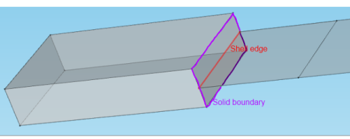
Type 1 connection: The shell connects to the solid in a thin region (having the same thickness as the shell), so that shell theory is valid on both sides. This connection is the most important from the application point of view and the most difficult to create manually.
Type 2 connection: The tangent plane to the shell is perpendicular to the face of a “thick” solid, in which case the physics of the connection can, at best, be approximate.
Type 3 connection: The shell acts as cladding on a solid.
The first two cases have similar physics and can be treated more or less as one case. Usually, the shell should not connect to parts on the solid boundary further away than what is represented by the shell thickness (or some other user-defined distance).
Shell Perpendicular to Solid
Figure 5-2 illustrates the first two cases. The shell edge can be part of the definition of the solid but there is no assumption about that.
Figure 5-2: An example of a shell extending perpendicular to the solid boundary.
The connection of a solid to a shell is based on that shell theory is valid on both sides of the connection. This can be divided into these assumptions:
One basic shell theory assumption is actually not valid in practice: plane sections do not always remain plane under deformation. A detailed analysis shows that if there is a transverse shear force in the section, there must be a deviation from planarity to get the correct shear strain distribution. This is more important as the shell grows thicker, but without it, it is not possible to get a perfect connection. In Mindlin plate theory, shear is related to the difference between rotation and the derivative of displacement, so that plane sections remain plane, but no longer perpendicular to the midsurface. This gives an average shear strain, while it is known from analytical solutions that the shear strain has a parabolic distribution through the thickness.
Consider a cut where the local coordinates are defined as follows:
x is the outward normal to the solid boundary
z is along the shell normal
y is the tangent to the shell edge, directed so that x-y-z form a right-hand system
Using the plane section assumption in the shell gives the displacements in the solid as:
where the subscripts sld and sh represent “solid” and “shell”, respectively, and a is the displacement of the shell normal, represented in the local directions.
The values on the solid boundaries should be interpreted as mapped using an extrusion operator from the shell edge.
A simple connection for the transverse direction can be generated by
This connection, however, enforces a ‘plane strain condition’ in the solid, which is not consistent with shell theory and which causes local unphysical stresses if Poisson’s ratio is nonzero. This effect disappears within a few elements from the connection, and the approximation can, in many situations, be acceptable. This constraint is enforced if Method is set to Rigid in the multiphysics coupling.
A more accurate connection is derived in the following. The first approximation of the stress state in a moderately curved shell is
where the relative thickness coordinate has been introduced.
Assuming that Hooke’s law and plane stress conditions are valid, the transverse direct strain can be computed as
The transverse displacement is then, after integration with respect to z:
Thus, in order to obtain a stress-free transverse displacement, this deformation must be allowed. Note that the last term makes the solid thinner on one side of the midsurface and thicker on the other. The constant term — that is, the displacement at the midsurface of the solid — is known from the shell midsurface displacement. The other two terms depend on the stress state and thus on derivatives of the displacement, which are not readily available. The K1 term is caused by the membrane action and the K2 term by the bending action.
For the transverse shear stress, Hooke’s law gives
which can be reformulated as
Note that as the K1 term is related to membrane action, it cannot contribute to the transverse shear stress. Since the derivative in the x direction cannot be controlled by a condition on the boundary, it is necessary to make an assumption about u(z′). An integration with respect to z gives
This shows that a third power of z is required in order to be able to represent the correct shear strain contribution.
It is, however, not possible to directly determine the coefficients in front of the additional terms, since they depend on the actual stress state. The idea is here to introduce them as dependent variables in the problem. These variables are defined by extra shape functions on the shell edge.
The constraints applied on the solid can then be written as
Here qu, qw1, and qw2 are the new dependent variables defined on the shell edge. They are dimensionless, due to the multiplication with the shell thickness, d. The constants ku = 3/5 and kw2 = 1/5 are explained below. The variable qw1 is proportional to the membrane axial strain, the variable qw2 is proportional to the bending strain, and the variable qu is proportional to the transverse shear strain. Since these variable are directly related to strains, the shape function order used is one order lower than for the displacements.
If no extra equations defining qu, qw1, and qw2 are introduced, these variables try to adapt to proper values through the reaction forces on the solid. The reaction force for u is the traction σx and the reaction force for w is the traction τxz. When taking the variation of the new dependent variables, these enforce the following constraints:
The equation with qw1 is trivially fulfilled because the shear stress is an even function of z. Inserting the known stress distributions gives equations that can be solved for ku and kw2.
The constraint expressions must now be formulated in global directions. As a start, the constraints are written on vector form in local directions as
(5-3)
where
The fact that az = 0 has been used when formulating Equation 5-3.
All coordinate directions are retrieved from the shell, because the normal to the solid boundary is not necessarily constant.
The only coordinate value needed is actually z. For the other two coordinates only the direction is important. The coordinate in the normal direction can be computed as
This definition of z assumes that the thickness of the solid does not change significantly. Under geometric nonlinearity, the computation should be based on the current geometry.
The latter expression introduces additional nonlinearities in the model because it depends on deformed position and deformed normal. Also, the position of the shell midsurface with respect to the solid is actually part of the solution.
Let Φ be the matrix that transforms displacements from the global system to the local system:
The expression for the constraints in global directions then becomes
The only transformation actually needed is thus the projection of the q vector. For a linear case, the transformation can be written as
where N is the undeformed shell normal (shell.an) and tl is the shell edge tangent (shell.tle). The coefficient s is either 1 or 1, and is selected so that the x direction coincides with the outward normal of the solid.
For a geometrically nonlinear case, the corresponding deformed directions are used.
When an offset is used for the shell, it is assumed that the center of the connection is at the actual shell midsurface.
Beam Perpendicular to Solid
This is the analogous case in 2D. Beam theory assumes that the stress in the out-of-plane direction is zero. It is thus only physically sound to connect to a model where the plane stress assumption is used. The derivation above still remains valid with the following exceptions: the displacements in the local y’ direction are zero and the tangent direction tl is replaced by the out-of-plane direction.
The shell thickness is replaced by twice the effective radius of the beam in the equations defining the displacements.
Shell Parallel to Solid
The case where the shell is parallel to the boundary of the solid exists in two versions — Shared and Parallel.
In the shared case, the shell is modeled on a boundary which is a face of the solid. In this case, it assumed that the names of the displacement degrees of freedom in the solid and shell interfaces are not the same. If the same names are used, there is no need to use a connection feature, since the coupling is then automatic. A shell offset can be used to model an actual distance between the boundaries. For a layer “glued” on the solid, the offset would equal half the shell thickness.
In the parallel case, a separate boundary is used for modeling the shell. The distance between the shell and the face of the solid is taken into account when setting up the constraints, so that
where ζ is a distance from the solid to the shell. The right hand side is mapped from the shell to the solid using an extrusion operator. The default is that ζ is half the shell thickness, but you can also use the geometrical distance between the boundaries, or a user-defined distance.
Connection Between Shells and Beams
When connecting elements from the Shell interface with elements from the Beam interface, the following must be noted:
You can create the appropriate couplings by adding a Solid-Thin Structure Connection multiphysics coupling. The theory of this connection is outlined below.
Beam Edge to Shell Edge
This coupling is intended for the common situation where beams are attached along a plate to act as stiffeners. There are two variants of the coupling:
The beam is modeled at an edge which is also an edge in the beam interface. This case is called Shell and beam shared edges in the Shell-Beam Connection node. In practice, the beam is usually placed on one side of the shell, and this offset plays an important role in the stiffness of the combined section. The offset, d0, can be given as a user input.
The beam is modeled at a separate edge, representing the actual centerline. This case is called Shell and beam parallel edges in the Shell-Beam Connection node, and the closest geometrical distance between the edges directly gives d0. You do not need to use the same mesh on both lines. Since the constraints are formed for the shell edge, some parts of the beams could however become unconnected if the beam elements are very short when compared to the shell element size.
The displacement at the centerline of the beam can then be written in therms of the degrees of freedom in the shell as
where n is the normal to the shell. The rotation vector in the beam can be expressed in the shell degrees of freedom as
For a geometrically linear case, the constraint
is enforced by the shell interface for each shell boundary. This is why there are only two active rotational degrees of freedom. To avoid propagating this constraint to the beam, only the those components of the beam that act in the plane of the shell should be constrained. This can be expressed as
which can be simplified to
The constraints are actually formed on the shell edge, and the degrees of freedom are taken from the beam using a General Extrusion operator which maps values from the closest point on the beam to the shell.
The definitions of n, t1, and t2 may however be discontinuous over a shell edge. For this reason, the constraint is formed using values from one boundary only if several boundaries share the edge. Another complications arises when the edge is a fold line, that is when the boundaries that meet do not have a common normal direction. On a fold line all three rotational degrees of freedom do exist in the shell and should then be connected to the corresponding degrees of freedom in the shell. In this case, also a third rotational constraint is formed.
Beam Point to Shell Boundary
This coupling is intended for the case when the beam is not in the same plane as the boundary modeled by shell theory. This case is called Shell boundaries to beam points in the Shell-Beam Connection node. Physically, this can be seen as a beam with one end welded to a plate. In order to get a correct stiffness representation of such a connection, it is necessary that the beam is connected to an area of the shell which is similar to the actual physical width of the beam. The connected area on the shell does not have to fit a boundary in the geometry. It is however necessary that the mesh size is such that there are at least three nodes within the connected area.
You can then select the region to connect using three different criteria.
The connected region is treated as rigid. The displacement of the shell is controlled by the displacement and rotation of the beam endpoint through
The coordinates of the shell are evaluated at the reference surface.
As it is only possible to constrain the in-plane rotations of the shell, the continuity in rotation is projected onto the shell, giving
The rotation of the beam around the normal of the shell, which does not participate in the rotation constraints, is indirectly connected through the displacement equation, so it implicitly receives an appropriate stiffness.
Beam Point to Shell Edge
This case is identical to the previous case, with the only exception that the selection in the Shell interface is an edge. The beam can have any orientation relative to the shell edge. This case is called Shell edges to beam points in the Shell-Beam Connection node.