The Semiclassical Model

Consider the motion of a wave packet, constructed using the functions Ψm(r) which modulate the Wannier functions. The wave function evolves according to Equation 3-33. Note that the perturbing potential, H1, is a function of position r and E0(-i∇) can be straightforwardly written as a function of the quantum mechanical momentum operator p=-i

∇. The equivalent classical Hamiltonian is H=E0(p)+H1(r) (where E0 is written as a function of p=

k). The quantity

k, which is analogous to the classical momentum in the Hamiltonian, is often referred to as the crystal momentum of the wave packet. The classical Hamiltonian results in classical particles that move according to the equations:

According to Ehrenfest’s theory (see Ref. 7 for a detailed discussion), the center of gravity of the wave packet moves in the same way as the corresponding classical Hamiltonian. Consequently the motion of a wave packet with associated charge -q, in a perturbing Hamiltonian of the form H1 = −qV moves according to the equations:

Here v(k) is the velocity of the wave packet, and F is the Lorentz force acting on it.

These equations are referred to as the semiclassical model (in the absence of magnetic fields). When magnetic fields are present Equation 3-35 takes the form:

(Ref. 1 provides references that derive this equation in full. Note also that Equation 3-34 is also modified in modern solid state theory to include an additional term due to the Berry curvature of the band. This term is usually zero for semiconducting materials of interest). The model is extremely successful to describe a range of practical transport phenomena.

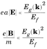
	The instantaneous velocity and momentum of a single electron fluctuates rapidly as it passes through the periodic potential of the crystal, so the crystal momentum is not directly related to the actual electron momentum and the wave packet velocity should be interpreted as an average drift velocity.

The semiclassical model is valid for wave packets that are localized to within greater than approximately ten lattice spacings. This restriction is apparent from the previous analysis but is also implied by the Heisenberg uncertainty principle Δx≈

/Δp≈1/kf where kf is the approximate magnitude of wave vectors at the Fermi surface. It would be unreasonable to use more than approximately 10% of the available states in a single wave packet. The wave packet is therefore large compared to the lattice size, and so sees only the average effect of the lattice.

Additionally, the physical size of the wave packets must be small compared to the length scale of electric or magnetic field variation. This is why the model is called semiclassical; the external fields are treated classically, but the periodic potential of the lattice is not. There is a further restriction on the local validity of the semiclassical model, which results from the fact that in the limit of zero periodic potential the classical limit should be recovered. In the classical limit the electron momentum and the crystal momentum become identical. At a given point in k-space the semiclassical equations are valid provided:

where a is of the order of the lattice constant, Ef is the Fermi energy, and Eg(k) is the energy difference to the nearest energy in a different band at the specified k-space point. In semiconductors the first condition is violated during electric breakdown, when electrons can make an interband transition driven by a large electric field. A similar phenomenon known as magnetic breakdown can occur in high magnetic fields. Although the semiclassical model really describes the transport of wave packets, conventionally the transport of electrons is discussed in the literature. This convention is therefore adopted from here onward.

The semiclassical model has important consequences for charge transport in materials. One of the more surprising consequences is that a filled band is completely inert. Since the semiclassical model does not allow intraband transitions, the electrons can only move between states within a band. Each state has a particular velocity associated with it (given by Equation 3-34) and electrons move between states according to Equation 3-35. In the reduced zone scheme, electrons that pass out of the Brillouin zone immediately reappear unchanged (except for a relabeling of the k-vector) at the opposite face. Summing the drift velocity over all the states in the band produces exactly the same result in the presence of applied fields as without them, since the band structure remains unchanged and since all the states are still occupied (see Ref. 1 for a formal derivation that integrates over all the states in a band). This result explains the existence of metals, insulators, and semiconductors. Metals are materials without a full band, in which an applied electric field can produce a large current. Insulators have a set of full bands and the Fermi energy lies within the band gap. The band gap is sufficiently large that the occupancy of the bands below the Fermi level is essentially one for all states at temperatures of interest. Similarly the band above the gap is essentially unoccupied in an insulator. Semiconductors are materials in which the Fermi level lies within the band gap, but in which the variation in the Fermi function overlaps the edges of adjacent bands at temperatures of interest, so that not all the states in the bands above (or below) the Fermi level are unoccupied (or occupied). This is why semiconductors usually have a higher resistance than metals since only a relatively small number of states in the band are unoccupied. The physics of semiconductor transport is determined by the band structure close to the top or the bottom of the bands adjacent to the Fermi level.

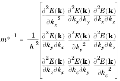
	In 3D the band gap must extend across all directions in k-space to produce a semiconductor or insulator.

Before considering how to compute the transport properties of bands that are not full, it is worth considering the implications of Equation 3-34 and Equation 3-35 for the relationship between force and electron velocity. In order to do so, the velocity must be related to the wave vector k. Therefore:

Note that both ∂v/∂k and

-2∂2E(k)/∂k2 are rank 2 tensors (matrices). Equation 3-36 defines the effective masses introduced in Equation 3-20.

In general, the effective mass matrix is defined as:

such that F = m* v. In Equation 3-20 the coordinate system for k' was chosen such that the m* matrix has zero for the off-diagonal terms. For an isotropic band m* is proportional to the identity matrix. In this instance, near the top of a band, it is easy to see that its value could be negative. Instead of thinking in terms of negative mass, it is more conventional to reverse the sign on the force and to consider a wave packet corresponding to a particle with positive charge and mass (this is known as a hole).

Finally consider the form of Equation 3-33 in the case where the band structure takes the form given by Equation 3-20. For simplicity consider the case of an isotropic effective mass so that:

Equation 3-33 now takes the form:

which is identical in form to the Schrödinger equation, except that the effective mass rather than the electron mass appears in the equation system. It is important to remember that for Equation 3-37 to apply the E–k relationship must be defined in an appropriate coordinate system. Note, however, that for the case of an anisotropic effective mass there are different coefficients for the derivatives in different directions in the Laplacian operator. Equation 3-37 also applies near the top of a band, so it is relevant for holes.