|
|
|
|
1
|
|
2
|
In the Select Physics tree, select Acoustics>Acoustic-Structure Interaction>Acoustic-Shell Interaction, Frequency Domain.
|
|
3
|
Click Add.
|
|
4
|
Click Study.
|
|
5
|
|
6
|
Click Done.
|
|
1
|
|
2
|
|
3
|
Click Browse.
|
|
4
|
Browse to the model’s Application Libraries folder and double-click the file vented_loudspeaker_enclosure.mphbin.
|
|
5
|
Click Import.
|
|
1
|
|
2
|
|
1
|
|
2
|
|
1
|
|
2
|
|
1
|
|
2
|
|
3
|
|
4
|
|
1
|
|
2
|
|
3
|
|
1
|
|
2
|
|
3
|
|
1
|
|
2
|
|
3
|
|
1
|
|
2
|
|
3
|
|
4
|
|
5
|
|
6
|
Click OK.
|
|
1
|
|
2
|
|
3
|
|
4
|
Click Browse.
|
|
5
|
Browse to the model’s Application Libraries folder and double-click the file vented_loudspeaker_enclosure_Rb.txt.
|
|
6
|
Click Import.
|
|
7
|
|
8
|
|
9
|
|
10
|
Locate the Interpolation and Extrapolation section. From the Extrapolation list, choose Nearest function.
|
|
1
|
|
2
|
|
3
|
|
4
|
Click Browse.
|
|
5
|
Browse to the model’s Application Libraries folder and double-click the file vented_loudspeaker_enclosure_Lb.txt.
|
|
6
|
Click Import.
|
|
7
|
|
8
|
|
9
|
|
10
|
Locate the Interpolation and Extrapolation section. From the Extrapolation list, choose Nearest function.
|
|
1
|
|
2
|
|
3
|
|
4
|
|
1
|
|
2
|
|
3
|
|
4
|
|
1
|
|
2
|
|
1
|
|
2
|
|
1
|
In the Model Builder window, under Component 1 (comp1) click Pressure Acoustics, Frequency Domain (acpr).
|
|
2
|
In the Settings window for Pressure Acoustics, Frequency Domain, locate the Domain Selection section.
|
|
3
|
|
1
|
|
2
|
|
3
|
|
1
|
|
2
|
|
3
|
In the tree, select Built-in>Air.
|
|
4
|
|
1
|
In the Model Builder window, under Component 1 (comp1) right-click Materials and choose Blank Material.
|
|
2
|
|
3
|
Locate the Geometric Entity Selection section. From the Geometric entity level list, choose Boundary.
|
|
4
|
|
5
|
|
1
|
|
2
|
|
3
|
Locate the Geometric Entity Selection section. From the Geometric entity level list, choose Boundary.
|
|
4
|
|
5
|
|
1
|
|
2
|
|
3
|
Locate the Geometric Entity Selection section. From the Geometric entity level list, choose Boundary.
|
|
4
|
|
5
|
|
1
|
|
2
|
In the tree, select Built-in>Copper.
|
|
3
|
|
4
|
|
1
|
|
2
|
|
3
|
|
1
|
|
2
|
|
3
|
|
4
|
|
5
|
|
1
|
In the Model Builder window, under Component 1 (comp1) right-click Pressure Acoustics, Frequency Domain (acpr) and choose Symmetry.
|
|
1
|
|
1
|
|
3
|
In the Settings window for Exterior Field Calculation, locate the Exterior Field Calculation section.
|
|
4
|
|
5
|
|
1
|
|
2
|
|
3
|
|
4
|
|
5
|
|
1
|
|
2
|
|
3
|
|
4
|
|
1
|
|
2
|
|
3
|
|
4
|
|
1
|
|
2
|
|
3
|
|
4
|
|
5
|
|
1
|
|
2
|
|
3
|
|
1
|
|
2
|
|
3
|
|
4
|
|
1
|
|
2
|
|
3
|
|
4
|
|
1
|
|
2
|
|
3
|
|
4
|
|
1
|
|
2
|
|
3
|
|
4
|
|
1
|
|
1
|
|
3
|
|
4
|
|
1
|
In the Model Builder window, under Component 1 (comp1) right-click Mesh 1 and choose Boundary Layers.
|
|
2
|
|
3
|
|
4
|
|
5
|
|
1
|
|
2
|
|
3
|
|
5
|
|
6
|
|
1
|
|
2
|
|
3
|
|
4
|
|
1
|
|
2
|
|
3
|
|
4
|
|
1
|
|
2
|
|
3
|
|
1
|
|
2
|
|
1
|
|
2
|
|
3
|
|
1
|
|
2
|
|
3
|
|
4
|
|
5
|
|
6
|
|
7
|
|
8
|
Click Replace.
|
|
1
|
|
2
|
|
3
|
In the Model Builder window, expand the Study 1>Solver Configurations>Solution 1 (sol1)>Stationary Solver 1 node.
|
|
4
|
Right-click Suggested Iterative Solver (GMRES with GMG and Direct Precon.) (asb1) and choose Enable.
|
|
5
|
|
1
|
|
2
|
|
3
|
|
4
|
|
5
|
|
6
|
|
1
|
|
2
|
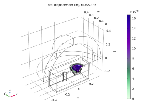
In the Settings window for Surface, click Replace Expression in the upper-right corner of the Expression section. From the menu, choose Component 1>Shell>Displacement>shell.disp - Total displacement - m.
|
|
1
|
|
2
|
|
3
|
|
4
|
|
5
|
|
6
|
|
1
|
|
2
|
|
3
|
|
4
|
|
5
|
|
6
|
|
1
|
|
2
|
|
3
|
|
1
|
|
2
|
|
3
|
|
1
|
|
2
|
|
3
|
|
4
|
Click Replace Expression in the upper-right corner of the Expression section. From the menu, choose Geometry>dom - Entity index.
|
|
5
|
|
6
|
|
7
|
|
8
|
|
1
|
|
2
|
|
3
|
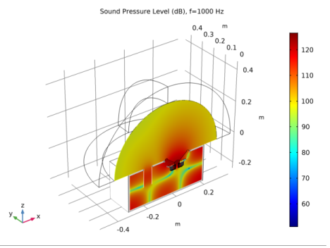
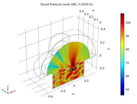
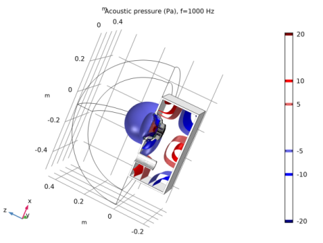
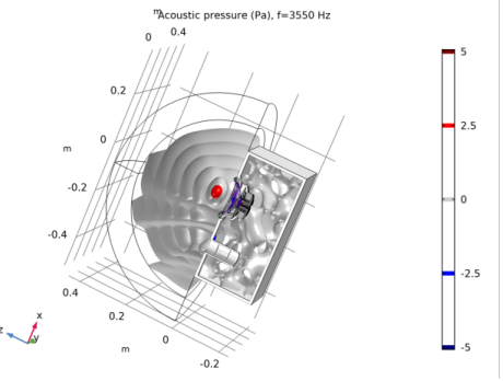
Locate the Title section. In the Title text area, type Sound Pressure Level (dB), f=eval(freq,Hz) Hz.
|
|
1
|
|
2
|
|
3
|
|
1
|
|
2
|
In the Settings window for Slice, click Replace Expression in the upper-right corner of the Expression section. From the menu, choose Component 1>Pressure Acoustics, Frequency Domain>Pressure and sound pressure level>acpr.Lp - Sound pressure level - dB.
|
|
3
|
|
4
|
|
5
|
|
6
|
|
1
|
|
2
|
|
1
|
|
2
|
|
3
|
|
4
|
|
1
|
|
2
|
|
3
|
|
4
|
|
5
|
|
6
|
|
7
|
|
1
|
|
2
|
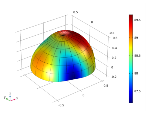
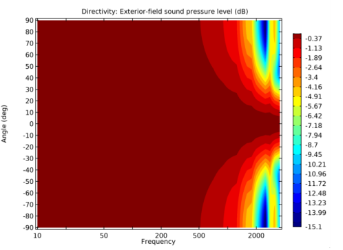
In the Settings window for 3D Plot Group, type Exterior-Field Sound Pressure Level in the Label text field.
|
|
3
|
|
4
|
|
1
|
|
2
|
|
3
|
|
4
|
|
5
|
Locate the Evaluation section. Find the Angles subsection. In the Number of elevation angles text field, type 30.
|
|
6
|
|
7
|
|
8
|
|
9
|
|
1
|
In the Model Builder window, right-click Exterior-Field Sound Pressure Level and choose Paste Volume.
|
|
2
|
|
3
|
|
1
|
|
2
|
|
3
|
|
4
|
|
5
|
|
6
|
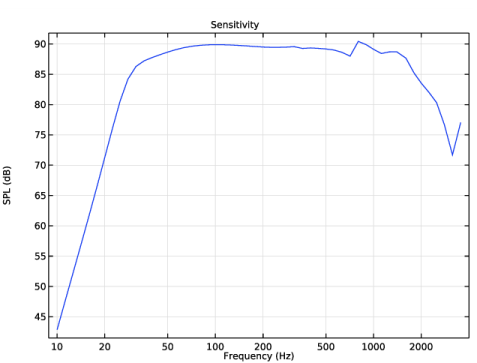
In the associated text field, type Frequency (Hz).
|
|
7
|
|
8
|
In the associated text field, type SPL (dB).
|
|
1
|
|
2
|
|
3
|
|
4
|
|
5
|
|
6
|
|
1
|
|
2
|
|
3
|
|
4
|
|
1
|
|
2
|
|
3
|
|
1
|
|
2
|
|
3
|
|
4
|
|
5
|
|
6
|
|
7
|
|
1
|
|
2
|
|
3
|
|
1
|
|
2
|
|
3
|
|
4
|
|
5
|
|
1
|
|
2
|
|
1
|
|
2
|
|
3
|
|
4
|
|
5
|
|
6
|
|
7
|
|
8
|
|
9
|
|
10
|
|
11
|
|
12
|
|
13
|