
|
|
|
|
•
|
|
1
|
|
2
|
|
3
|
Click Add.
|
|
4
|
In the Select Physics tree, select Acoustics>Acoustic-Structure Interaction>Acoustic-Solid Interaction, Frequency Domain.
|
|
5
|
Click Add.
|
|
6
|
Click Study.
|
|
7
|
|
8
|
Click Done.
|
|
1
|
|
2
|
Browse to the model’s Application Libraries folder and double-click the file loudspeaker_driver_geom_sequence.mph.
|
|
3
|
|
4
|
|
1
|
|
2
|
|
1
|
|
2
|
|
1
|
|
1
|
|
2
|
|
3
|
In the tree, select Built-in>Air.
|
|
4
|
|
5
|
|
6
|
|
1
|
|
3
|
|
1
|
In the Material Browser window, In the ribbon make sure to select the Materials tab and then click the Browse Materials icon.
|
|
2
|
|
3
|
Browse to the model’s Application Libraries folder and double-click the file loudspeaker_driver_materials.mph.
|
|
4
|
Click Done.
|
|
1
|
|
2
|
|
3
|
|
4
|
|
5
|
|
6
|
|
7
|
|
8
|
|
9
|
|
10
|
|
11
|
|
12
|
|
13
|
|
14
|
|
1
|
|
1
|
|
1
|
|
1
|
|
1
|
|
1
|
|
1
|
|
1
|
|
3
|
|
4
|
|
5
|
Specify the e vector as
|
|
1
|
|
3
|
|
4
|
|
1
|
|
2
|
|
3
|
|
4
|
|
5
|
|
6
|
|
7
|
|
8
|
|
1
|
In the Model Builder window, under Component 1 (comp1) click Pressure Acoustics, Frequency Domain (acpr).
|
|
1
|
|
3
|
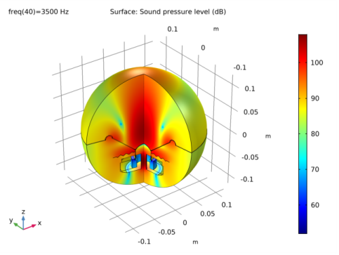
In the Settings window for Exterior Field Calculation, locate the Exterior Field Calculation section.
|
|
4
|
|
1
|
|
1
|
|
2
|
|
3
|
|
5
|
|
1
|
|
2
|
|
3
|
|
5
|
|
1
|
|
2
|
|
3
|
|
5
|
|
1
|
|
1
|
|
2
|
|
3
|
|
1
|
|
2
|
|
3
|
|
1
|
|
3
|
|
4
|
|
1
|
|
2
|
|
3
|
|
1
|
|
2
|
|
3
|
|
5
|
|
6
|
|
7
|
|
1
|
|
2
|
|
3
|
|
1
|
|
2
|
|
3
|
|
4
|
|
5
|
|
6
|
|
7
|
|
1
|
|
2
|
|
3
|
|
1
|
|
2
|
|
3
|
In the table, clear the Solve for check box for Pressure Acoustics, Frequency Domain (acpr) and Solid Mechanics (solid).
|
|
1
|
|
2
|
|
3
|
|
4
|
Locate the Physics and Variables Selection section. In the table, clear the Solve for check box for Pressure Acoustics, Frequency Domain (acpr) and Solid Mechanics (solid).
|
|
5
|
|
1
|
|
2
|
|
3
|
|
1
|
|
2
|
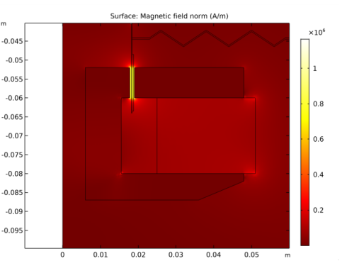
In the Settings window for Surface, click Replace Expression in the upper-right corner of the Expression section. From the menu, choose Component 1>Magnetic Fields>Magnetic>mf.normH - Magnetic field norm - A/m.
|
|
3
|
|
4
|
|
1
|
|
2
|
|
1
|
|
2
|
|
3
|
|
4
|
|
1
|
|
2
|
|
3
|
|
4
|
|
5
|
Locate the Expressions section. In the table, enter the following settings:
|
|
6
|
|
7
|
Click Evaluate.
|
|
1
|
|
2
|
|
1
|
|
2
|
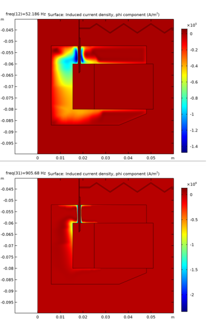
In the Settings window for Surface, click Replace Expression in the upper-right corner of the Expression section. From the menu, choose Component 1>Magnetic Fields>Currents and charge>Induced current density (spatial frame) - A/m²>mf.Jiphi - Induced current density, phi component.
|
|
3
|
|
1
|
|
2
|
|
3
|
|
4
|
|
5
|
|
1
|
|
2
|
|
1
|
|
2
|
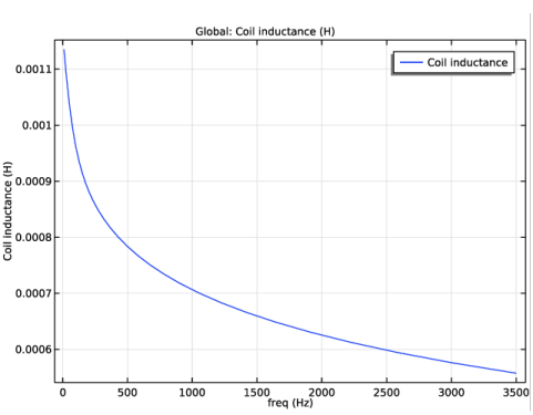
In the Settings window for Global, click Replace Expression in the upper-right corner of the y-axis data section. From the menu, choose Component 1>Magnetic Fields>Coil parameters>mf.LCoil_1 - Coil inductance - H.
|
|
3
|
|
1
|
|
1
|
|
2
|
|
3
|
|
4
|
|
5
|
|
1
|
|
2
|
|
1
|
In the Model Builder window, under Magnetic Fields Study, Ctrl-click to select Step 1: Stationary and Step 2: Frequency Domain Perturbation.
|
|
2
|
Right-click and choose Copy.
|
|
1
|
|
2
|
|
3
|
|
1
|
|
2
|
In the Settings window for Frequency Domain Perturbation, locate the Physics and Variables Selection section.
|
|
4
|
|
1
|
|
2
|
|
3
|
|
4
|
|
5
|
|
1
|
|
2
|
|
3
|
|
4
|
|
5
|
|
1
|
|
2
|
|
1
|
|
2
|
|
3
|
|
4
|
|
5
|
|
1
|
|
2
|
|
3
|
|
4
|
|
5
|
|
6
|
|
1
|
|
2
|
|
1
|
|
2
|
|
3
|
|
4
|
|
1
|
|
2
|
|
3
|
|
4
|
|
5
|
|
6
|
|
7
|
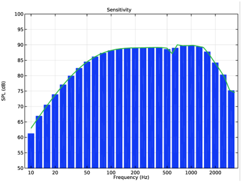
In the associated text field, type Frequency (Hz).
|
|
8
|
|
9
|
In the associated text field, type SPL (dB).
|
|
1
|
|
2
|
|
3
|
|
4
|
|
5
|
|
6
|
|
1
|
|
2
|
|
3
|
|
4
|
|
5
|
|
1
|
|
2
|
|
3
|
|
4
|
|
5
|
|
6
|
|
1
|
|
2
|
|
3
|
|
4
|
|
5
|
|
6
|
|
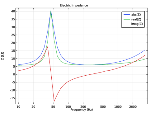
7
|
In the associated text field, type Frequency (Hz).
|
|
8
|
|
9
|
In the associated text field, type Z (\Omega).
|
|
1
|
|
2
|
|
4
|
|
5
|
|
1
|
|
2
|
|
1
|
|
2
|
|
3
|
|
1
|
|
2
|
|
1
|
In the Model Builder window, under Results>Datasets right-click Complete Study/Solution 3 (sol3) and choose Duplicate.
|
|
2
|
|
3
|
|
1
|
|
2
|
|
3
|
|
1
|
|
2
|
|
3
|
|
4
|
|
5
|
|
6
|
|
7
|
|
1
|
|
2
|
|
3
|
|
4
|
Click to expand the Layers section. In the table, enter the following settings:
|
|
1
|
|
2
|
|
3
|
|
4
|
|
5
|
|
6
|
Locate the Layers section. In the table, enter the following settings:
|
|
1
|
|
2
|
|
3
|
|
4
|
On the object c2, select Boundaries 2–4 only.
|
|
1
|
|
2
|
|
3
|
|
4
|
|
5
|
|
6
|
|
1
|
|
2
|
Select the object c1 only.
|
|
3
|
|
4
|
|
5
|
Select the object r1 only.
|
|
1
|
|
2
|
|
3
|
|
4
|
|
5
|
|
6
|
|
1
|
|
2
|
|
3
|
|
4
|
|
5
|
|
6
|
|
1
|
|
2
|
|
3
|
|
4
|
|
5
|
|
6
|
|
1
|
|
2
|
|
3
|
|
4
|
|
5
|
|
6
|
|
7
|
|
1
|
|
2
|
|
3
|
|
4
|
|
5
|
|
1
|
|
2
|
|
3
|
|
4
|
Select the object r2 only.
|
|
5
|
Locate the Difference section. Find the Objects to subtract subsection. Select the Activate selection toggle button.
|
|
6
|
|
1
|
|
2
|
|
3
|
|
4
|
|
5
|
|
6
|
|
7
|
|
1
|
|
2
|
|
3
|
|
4
|
|
5
|
|
6
|
|
7
|
|
1
|
|
2
|
|
3
|
|
4
|
|
5
|
|
6
|
|
1
|
|
2
|
|
3
|
|
4
|
|
5
|
|
6
|
|
1
|
|
2
|
|
3
|
|
4
|
In the r text field, type 23[mm] 26[mm] 26[mm] 32[mm] 32[mm] 38[mm] 38[mm] 44[mm] 44[mm] 50[mm] 50[mm] 56[mm] 56[mm] 59[mm] 59[mm] 59[mm] 59[mm] 56[mm] 56[mm] 50[mm] 50[mm] 44[mm] 44[mm] 38[mm] 38[mm] 32[mm] 32[mm] 26[mm] 26[mm] 23[mm] 23[mm] 23[mm].
|
|
5
|
In the z text field, type -44.1[mm] -42.1[mm] -42.1[mm] -46.1[mm] -46.1[mm] -42.1[mm] -42.1[mm] -46.1[mm] -46.1[mm] -42.1[mm] -42.1[mm] -46.1[mm] -46.1[mm] -44.1[mm] -44.1[mm] -44.5[mm] -44.5[mm] -46.5[mm] -46.5[mm] -42.5[mm] -42.5[mm] -46.5[mm] -46.5[mm] -42.5[mm] -42.5[mm] -46.5[mm] -46.5[mm] -42.5[mm] -42.5[mm] -44.5[mm] -44.5[mm] -44.1.
|
|
1
|
|
2
|
|
3
|
|
4
|
|
5
|
|
1
|
|
2
|
|
3
|
|
4
|
|
5
|
Click OK.
|
|
6
|
|
7
|
|
8
|
|
9
|
|
1
|
|
2
|
|
3
|
|
4
|
Locate the Layers section. In the table, enter the following settings:
|
|
5
|
|
6
|
|
1
|
|
2
|
On the object c3, select Boundaries 1 and 2 only.
|
|
1
|
|
2
|
|
3
|
|
4
|
|
5
|
|
6
|
|
1
|
|
2
|
|
1
|
|
2
|
|
3
|
|
4
|
On the object uni2, select Domains 2–5 only.
|
|
5
|
Locate the Selections of Resulting Entities section. Find the Cumulative selection subsection. From the Contribute to list, choose Composite.
|
|
6
|
