|
|
|
|
•
|
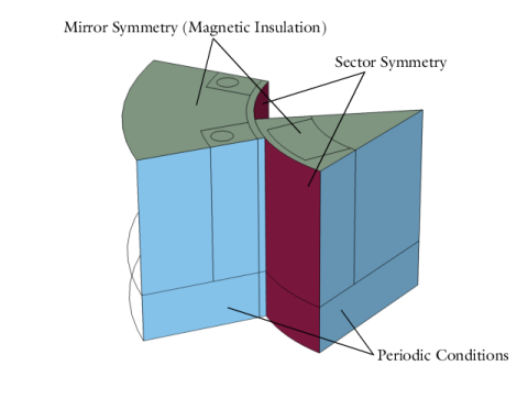
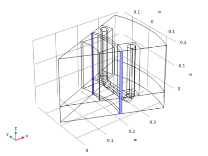
Periodic Boundary Conditions must be used on the sides of the sector symmetry. The type of periodicity chosen is Antiperiodicity, since the inputs to the model (the remanent flux density in the permanent magnets) change sign in adjacent sectors.
|
|
•
|
The Sector Symmetry pair condition is applied on the identity pair created by the geometry at the contact boundary between rotor and stator. The type of periodicity must match the type specified in the Periodic Boundary Condition features, that is, Antiperiodicity.
|
|
•
|
|
•
|
The vector potential formulation is subject to gauge freedom, meaning that the solution is unique up to a gauge transformation. To ensure a globally unique solution, it is necessary to choose (fix) the gauge by using the Gauge Fixing for A-Field feature in all domains where the vector formulation is used. More information about the electromagnetic gauge and gauge fixing can be found in the AC/DC Module User’s Guide.
|
|
1
|
|
2
|
In the Select Physics tree, select AC/DC>Electromagnetics and Mechanics>Rotating Machinery, Magnetic (rmm).
|
|
3
|
Click Add.
|
|
4
|
Click Study.
|
|
5
|
In the Select Study tree, select Preset Studies for Selected Physics Interfaces>Coil Geometry Analysis.
|
|
6
|
Click Done.
|
|
1
|
|
2
|
|
1
|
|
2
|
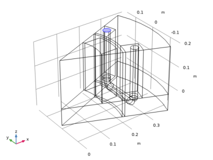
Browse to the model’s Application Libraries folder and double-click the file sector_generator_3d_geom_sequence.mph.
|
|
3
|
|
4
|
|
1
|
|
2
|
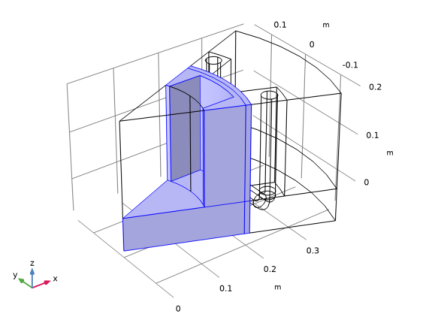
In the Model Builder window, expand the Component 1 (comp1)>Definitions node, then click Explicit 1.
|
|
3
|
|
4
|
|
1
|
|
2
|
|
1
|
|
2
|
|
1
|
|
2
|
|
3
|
|
4
|
|
5
|
Click OK.
|
|
1
|
|
2
|
|
3
|
|
1
|
|
2
|
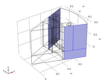
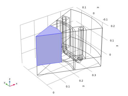
In the Settings window for Explicit, type Periodic Condition: Stator, Scalar Potential in the Label text field.
|
|
3
|
|
1
|
|
2
|
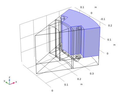
In the Settings window for Explicit, type Periodic Condition: Stator, Vector Potential in the Label text field.
|
|
3
|
|
1
|
|
2
|
|
3
|
In the tree, select Built-in>Air.
|
|
4
|
|
5
|
|
6
|
|
7
|
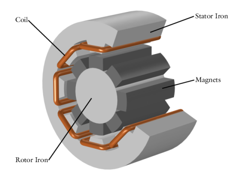
In the tree, select AC/DC>Hard Magnetic Materials>Sintered NdFeB Grades (Chinese Standard)>N50 (Sintered NdFeB).
|
|
8
|
|
9
|
|
1
|
In the Model Builder window, under Component 1 (comp1)>Materials click Soft Iron (Without Losses) (mat2).
|
|
1
|
|
2
|
|
3
|
|
1
|
In the Model Builder window, under Component 1 (comp1) right-click Rotating Machinery, Magnetic (rmm) and choose Magnetic Flux Conservation.
|
|
2
|
In the Settings window for Magnetic Flux Conservation, type Magnetic Flux Conservation: Air Gap in the Label text field.
|
|
1
|
|
3
|
In the Settings window for Magnetic Flux Conservation, locate the Constitutive Relation B-H section.
|
|
4
|
|
5
|
|
6
|
Locate the Constitutive Relation B-H section. From the || B r || list, choose User defined. In the associated text field, type 1.4.
|
|
1
|
|
2
|
In the Settings window for Magnetic Flux Conservation, type Magnetic Flux Conservation: Rotor Iron in the Label text field.
|
|
4
|
|
1
|
|
2
|
|
4
|
|
1
|
|
3
|
|
4
|
|
5
|
|
6
|
|
7
|
|
8
|
|
9
|
|
1
|
|
2
|
|
3
|
|
1
|
|
1
|
|
1
|
|
2
|
|
3
|
In the Show More Options dialog box, in the tree, select the check box for the node Physics>Advanced Physics Options.
|
|
4
|
Click OK.
|
|
5
|
|
6
|
|
7
|
|
1
|
|
1
|
|
2
|
|
3
|
|
4
|
|
5
|
Click OK.
|
|
6
|
|
7
|
|
8
|
|
9
|
|
1
|
|
2
|
|
3
|
|
4
|
|
1
|
|
2
|
|
3
|
|
4
|
|
1
|
|
2
|
|
3
|
|
4
|
|
1
|
|
2
|
|
3
|
|
4
|
|
5
|
|
6
|
|
1
|
|
2
|
In the Settings window for Rotating Machinery, Magnetic, click to expand the Discretization section.
|
|
3
|
|
4
|
|
1
|
|
2
|
|
1
|
|
2
|
|
3
|
|
1
|
|
2
|
|
3
|
|
4
|
|
5
|
|
6
|
|
7
|
|
8
|
Find the Algebraic variable settings subsection. From the Error estimation list, choose Exclude algebraic.
|
|
9
|
|
10
|
|
11
|
|
12
|
|
1
|
|
2
|
|
3
|
|
1
|
|
2
|
|
3
|
|
1
|
|
2
|
|
1
|
|
2
|
|
3
|
|
4
|
|
1
|
|
2
|
|
3
|
|
1
|
|
2
|
|
1
|
|
2
|
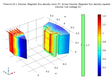
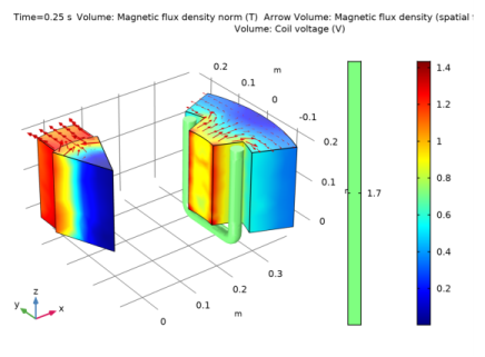
In the Settings window for Arrow Volume, click Replace Expression in the upper-right corner of the Expression section. From the menu, choose Component 1>Rotating Machinery, Magnetic (Magnetic Fields)>Magnetic>rmm.Bx,...,rmm.Bz - Magnetic flux density (spatial frame).
|
|
3
|
Locate the Arrow Positioning section. Find the x grid points subsection. In the Points text field, type 20.
|
|
4
|
|
5
|
|
6
|
|
1
|
|
2
|
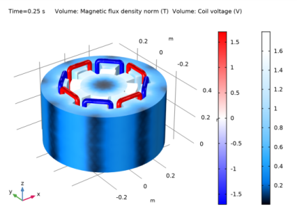
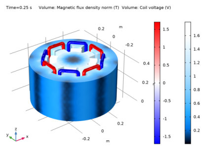
In the Settings window for Volume, click Replace Expression in the upper-right corner of the Expression section. From the menu, choose Component 1>Rotating Machinery, Magnetic (Magnetic Fields)>Coil parameters>rmm.VCoil_1 - Coil voltage - V.
|
|
3
|
|
4
|
|
5
|
|
1
|
|
2
|
|
3
|
|
4
|
|
1
|
|
2
|
|
3
|
|
4
|
|
5
|
|
1
|
|
2
|
|
3
|
|
4
|
|
5
|
|
1
|
|
2
|
|
3
|
|
4
|
|
5
|
|
1
|
|
2
|
|
3
|
|
4
|
|
5
|
|
1
|
|
2
|
|
1
|
|
2
|
|
3
|
|
4
|
|
1
|
|
2
|
In the Settings window for Volume, click Replace Expression in the upper-right corner of the Expression section. From the menu, choose Component 1>Rotating Machinery, Magnetic (Magnetic Fields)>Coil parameters>rmm.VCoil_1 - Coil voltage - V.
|
|
3
|
|
4
|
|
1
|
|
2
|
|
3
|
|
1
|
|
2
|
|
1
|
|
2
|
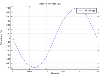
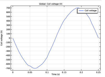
In the Settings window for Global, click Replace Expression in the upper-right corner of the y-axis data section. From the menu, choose Component 1>Rotating Machinery, Magnetic (Magnetic Fields)>Coil parameters>rmm.VCoil_1 - Coil voltage - V.
|
|
3
|
|
1
|
|
2
|
|
3
|
|
4
|
|
5
|