|
|
|

|
1
|
|
2
|
|
3
|
Click Add.
|
|
4
|
Click Study.
|
|
5
|
|
6
|
Click Done.
|
|
1
|
|
2
|
|
1
|
|
2
|
|
3
|
|
4
|
Click to expand the Layers section. In the table, enter the following settings:
|
|
1
|
|
2
|
|
3
|
|
4
|
|
1
|
|
2
|
|
3
|
|
4
|
|
5
|
|
1
|
|
3
|
|
4
|
|
1
|
|
2
|
|
3
|
In the tree, select Built-in>Air.
|
|
4
|
|
5
|
|
1
|
In the Model Builder window, under Component 1 (comp1) right-click Magnetic Fields (mf) and choose External Current Density.
|
|
3
|
|
4
|
|
1
|
|
3
|
|
4
|
|
1
|
|
3
|
|
4
|
|
1
|
|
3
|
|
4
|
|
1
|
|
1
|
|
2
|
|
3
|
|
4
|
Click to expand the Element Size Parameters section. In the Maximum element size text field, type 0.2.
|
|
5
|
|
1
|
|
2
|
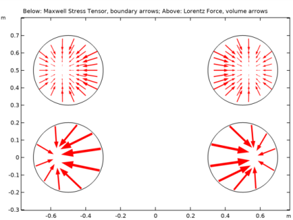
In the Settings window for Arrow Line, click Replace Expression in the upper-right corner of the Expression section. From the menu, choose Component 1>Magnetic Fields>Mechanical>mf.nTx_wire1,mf.nTy_wire1 - Maxwell surface stress tensor.
|
|
3
|
|
4
|
|
5
|
|
6
|
|
7
|
|
1
|
|
2
|
In the Settings window for Arrow Line, click Replace Expression in the upper-right corner of the Expression section. From the menu, choose Component 1>Magnetic Fields>Mechanical>mf.nTx_wire2,mf.nTy_wire2 - Maxwell surface stress tensor.
|
|
3
|
|
4
|
|
5
|
|
6
|
|
1
|
|
2
|
In the Settings window for Global Evaluation, click Replace Expression in the upper-right corner of the Expressions section. From the menu, choose Component 1>Magnetic Fields>Mechanical>Electromagnetic force - N>mf.Forcex_wire1 - Electromagnetic force, x component.
|
|
3
|
Click Evaluate.
|
|
1
|
Go to the Table window.
|
|
2
|
In the Settings window for Global Evaluation, click Replace Expression in the upper-right corner of the Expressions section. From the menu, choose Component 1>Magnetic Fields>Mechanical>Electromagnetic force - N>mf.Forcex_wire2 - Electromagnetic force, x component.
|
|
3
|
Click Evaluate.
|
|
4
|
Go to the Table window.
|
|
1
|
|
3
|
In the Settings window for Surface Integration, click Replace Expression in the upper-right corner of the Expressions section. From the menu, choose Component 1>Magnetic Fields>Mechanical>Lorentz force contribution, instantaneous value - N/m³>mf.FLtzix - Lorentz force contribution, instantaneous value, x component.
|
|
4
|
Click Evaluate.
|
|
1
|
Go to the Table window.
|
|
3
|
Click Evaluate.
|
|
1
|
|
1
|
|
2
|
|
3
|
|
1
|
In the Model Builder window, expand the Component 1 (comp1)>Meshes>Mesh 2>Mapped 1 node, then click Component 1 (comp1)>Meshes>Mesh 2>Distribution 1.
|
|
2
|
|
3
|
|
1
|
|
2
|
|
3
|
|
4
|
|
5
|
|
1
|
|
2
|
|
3
|
Click Add.
|
|
4
|
|
5
|
Click Range.
|
|
6
|
|
7
|
|
8
|
|
9
|
Click Replace.
|
|
1
|
|
1
|
|
2
|
|
3
|
|
1
|
|
2
|
|
4
|
|
5
|
|
6
|
|
7
|
|
8
|
|
9
|
|
1
|
|
2
|
|
3
|
|
4
|
|
5
|
|
6
|
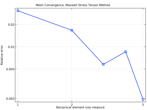
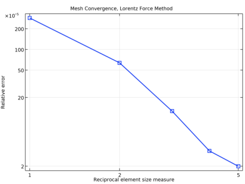
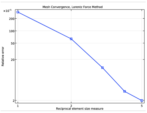
In the associated text field, type Reciprocal element size measure.
|
|
7
|
|
8
|
In the associated text field, type Relative error.
|
|
9
|
|
1
|
|
2
|
|
3
|
|
4
|
|
1
|
In the Model Builder window, right-click Mesh Convergence, Maxwell Stress Tensor Method and choose Duplicate.
|
|
2
|
|
3
|
|
4
|
|
1
|
In the Model Builder window, expand the Results>Mesh Convergence, Lorentz Force Method node, then click Global 1.
|
|
2
|
|
1
|
|
2
|
|
1
|
|
2
|
In the Settings window for 2D Plot Group, type Compared visualization of Lorenz Force and Maxwell Stress tensor in the Label text field.
|
|
3
|
|
4
|
|
6
|
|
1
|
|
2
|
|
3
|
|
4
|
|
5
|
|
6
|
|
1
|
|
2
|
|
3
|
|
4
|
|
5
|
|
1
|
In the Model Builder window, click Compared visualization of Lorenz Force and Maxwell Stress tensor.
|
|
2
|
|
3
|
|
4
|
In the Title text area, type Below: Maxwell Stress Tensor, boundary arrows; Above: Lorentz Force, volume arrows.
|
|
1
|
|
2
|
|
3
|
|
4
|
|
5
|
|
6
|
|
7
|
|
1
|
Right-click Compared visualization of Lorenz Force and Maxwell Stress tensor and choose Arrow Surface.
|
|
2
|
In the Settings window for Arrow Surface, click Replace Expression in the upper-right corner of the Expression section. From the menu, choose Component 1>Magnetic Fields>Mechanical>mf.FLtzix,mf.FLtziy - Lorentz force contribution, instantaneous value.
|
|
3
|
Locate the Arrow Positioning section. Find the X grid points subsection. In the Points text field, type 21.
|
|
4
|
|
5
|
|
6
|
|
1
|
|
2
|
|
3
|
|
4
|
|
5
|
|
1
|
In the Model Builder window, click Compared visualization of Lorenz Force and Maxwell Stress tensor.
|
|
2
|
|
3
|