PDF

Eddy Currents
Introduction
Induced eddy currents and associated thermal loads are of interest in many high power AC applications. This example is of general nature and illustrates some of the involved physics as well as suitable modeling techniques in the AC/DC Module.
Model Definition
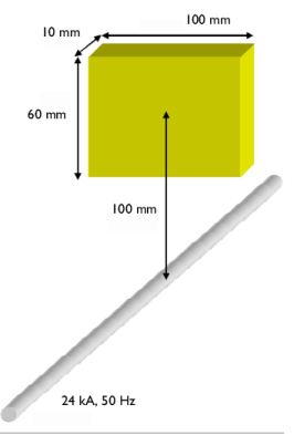
A metallic plate is placed near a 50 Hz AC conductor. The resulting eddy current distribution in the plate depends on the conductivity and permeability of the plate. The discussion considers four different materials: copper, aluminum, stainless steel, and magnetic iron. The step-by-step instructions focus on copper and iron. The geometry consists of a single wire and a plate with dimensions as shown below.
Because one cannot afford meshing an infinite volume, it is necessary to specify a finite volume to mesh and solve for. In this case, it makes sense to enclose the wire and the plate in a cylinder with the wire on the axis of this cylinder. This is a good choice when used with the default boundary condition, Magnetic Insulation. This condition forces the field to be tangential to the exterior boundaries. For the cylindrical shape of the domain that is a reasonable approximation to reality.
The conductor is modeled as a line current with 0° phase and an effective (RMS) value of 24 kA.
The magnetic vector potential is calculated from
where σ is the conductivity, ε the permittivity, and μ the permeability.
An important parameter in eddy current modeling is the skin depth, δ.
The following table lists the skin depth for the different materials at a frequency of 50 Hz.
In order for the model to produce accurate results, the mesh needs to resolve the evanescent fields in the metal. In practice, this means you need to resolve the skin depth with at least a bit more than 1 element, preferably closer to 2 or even more. This application uses a maximum element size of 5 mm for the copper plate.
When the skin depth is small in comparison to the size of the conducting objects, it can be practically impossible to resolve the skin depth. This often happens at high frequencies, in large structures, or with highly conductive and permeable materials. These cases require a different technique: Exclude the interior of the conducting objects from the model. Instead, represent them with an impedance boundary condition. This condition essentially sets the skin depth to zero, making all induced currents flow on the surface of the conductors. Mathematically, the relation between the magnetic and electric field at the boundary reads:
The dissipated power density, Pd (SI unit: W/m2) can be calculated from
where JS is the induced surface current density, and the asterisk (*) denotes the complex conjugate.
This model has the interior of the plate included in the model for copper, and uses the impedance boundary condition for magnetic iron.
Results and Discussion
The induced eddy current distribution for a plate made of copper is shown as streamlines, whereas the distribution of the ohmic losses is shown as a slice plot.
A total dissipated power of 6 W was obtained from integration through the plate. If you repeat the simulation for different materials, the application shows that lowering the conductivity decreases the dissipated power. However, for high permeability materials like soft iron, the dissipated power is higher than in copper (27 W) despite a much lower conductivity.
Application Library path: ACDC_Module/Inductive_Devices_and_Coils/eddy_currents
Modeling Instructions
From the File menu, choose New.
New
In the New window, click Model Wizard.
Model Wizard
1
In the Model Wizard window, click 3D.
2
In the Select Physics tree, select AC/DC>Electromagnetic Fields>Magnetic Fields (mf).
3
Click Add.
4
Click Study.
5
In the Select Study tree, select General Studies>Frequency Domain.
6
Click Done.
Geometry 1
1
In the Model Builder window, under Component 1 (comp1) click Geometry 1.
2
In the Settings window for Geometry, locate the Units section.
3
From the Length unit list, choose mm.
Cylinder 1 (cyl1)
1
In the Geometry toolbar, click Cylinder.
2
In the Settings window for Cylinder, locate the Size and Shape section.
3
In the Radius text field, type 250.
4
In the Height text field, type 300.
5
Locate the Axis section. From the Axis type list, choose Cartesian.
6
In the x text field, type 1.
7
In the z text field, type 0.
Line Segment 1 (ls1)
1
In the Geometry toolbar, click More Primitives and choose Line Segment.
2
In the Settings window for Line Segment, locate the Starting Point section.
3
From the Specify list, choose Coordinates.
4
Locate the Endpoint section. From the Specify list, choose Coordinates.
5
In the x text field, type 300.
6
Click Build All Objects.
Block 1 (blk1)
1
In the Geometry toolbar, click Block.
2
In the Settings window for Block, locate the Size and Shape section.
3
In the Width text field, type 10.
4
In the Depth text field, type 100.
5
In the Height text field, type 60.
6
Locate the Position section. In the x text field, type 145.
7
In the y text field, type -50.
8
In the z text field, type 70.
9
Click Build All Objects.
10
Click the Transparency button in the Graphics toolbar.
The model geometry is now complete. Prepare your simulation by defining selection groups.
Definitions
Explicit 1
1
In the Definitions toolbar, click Explicit.
2
Right-click Explicit 1 and choose Rename.
3
In the Rename Explicit dialog box, type Plate in the New label text field.
4
5
Explicit 2
1
In the Definitions toolbar, click Explicit.
2
In the Model Builder window, right-click Explicit 2 and choose Rename.
3
In the Rename Explicit dialog box, type Plate Boundaries in the New label text field.
4
5
6
In the Settings window for Explicit, locate the Output Entities section.
7
From the Output entities list, choose Adjacent boundaries.
Add Material
1
In the Home toolbar, click Add Material to open the Add Material window.
2
Go to the Add Material window.
3
4
Click Add to Component in the window toolbar.
Materials
Air (mat1)
1
In the Settings window for Material, locate the Material Contents section.
2
Note that a small nonzero value of the air conductivity will not substantially affect the results, but it will help the solver to converge.
Next, override Air as the material for the plate domain by Copper.
Add Material
1
Go to the Add Material window.
2
In the tree, select Built-in>Copper.
3
Click Add to Component in the window toolbar.
4
In the Home toolbar, click Add Material to close the Add Material window.
Materials
Copper (mat2)
1
In the Settings window for Material, locate the Geometric Entity Selection section.
2
From the Selection list, choose Plate.
Magnetic Fields (mf)
Edge Current 1
1
In the Model Builder window, under Component 1 (comp1) right-click Magnetic Fields (mf) and choose Edges>Edge Current.
2
3
In the Settings window for Edge Current, locate the Edge Current section.
4
In the I0 text field, type sqrt(2)*24[kA], resulting in an RMS current of 24 kA.
Mesh 1
To resolve the skin depth while maintaining a good mesh economy, mesh the copper plate finer than the rest of the geometry. Note that you need to add the finer mesh first in the sequence; otherwise you would get a coarse mesh on the common domain boundaries that would constrain the mesh inside the copper plate domain.
Free Tetrahedral 1
1
In the Model Builder window, under Component 1 (comp1) right-click Mesh 1 and choose Free Tetrahedral.
2
In the Settings window for Free Tetrahedral, locate the Domain Selection section.
3
From the Geometric entity level list, choose Domain.
4
From the Selection list, choose Plate.
5
Click to expand the Scale Geometry section. In the y-direction scale text field, type 0.4.
6
In the z-direction scale text field, type 0.4.
Size 1
1
Right-click Free Tetrahedral 1 and choose Size.
2
In the Settings window for Size, locate the Element Size section.
3
Click the Custom button.
4
Locate the Element Size Parameters section. Select the Maximum element size check box.
5
Free Tetrahedral 2
1
In the Model Builder window, right-click Mesh 1 and choose Free Tetrahedral.
2
In the Settings window for Mesh, click Build All.
Study 1
Step 1: Frequency Domain
1
In the Model Builder window, under Study 1 click Step 1: Frequency Domain.
2
In the Settings window for Frequency Domain, locate the Study Settings section.
3
In the Frequencies text field, type 50.
4
In the Home toolbar, click Compute.
Results
Magnetic Flux Density Norm (mf)
The default plot shows the magnetic flux density norm in three cross sections. The following instructions show you how to visualize the eddy currents and the resistive heating in the copper plate.
Multislice 1
1
In the Model Builder window, expand the Magnetic Flux Density Norm (mf) node.
2
Right-click Multislice 1 and choose Delete. Click Yes to confirm.
Slice 1
1
In the Model Builder window, right-click Magnetic Flux Density Norm (mf) and choose Slice.
2
In the Settings window for Slice, click Replace Expression in the upper-right corner of the Expression section. From the menu, choose Component 1>Magnetic Fields>Heating and losses>mf.Qrh - Volumetric loss density, electric - W/m³.
3
Locate the Plane Data section. From the Entry method list, choose Coordinates.
4
In the X-coordinates text field, type 145.1.
5
In the Magnetic Flux Density Norm (mf) toolbar, click Plot.
6
Click the Transparency button in the Graphics toolbar. This returns the transparency setting to its default state.
Streamline 1
1
Right-click Magnetic Flux Density Norm (mf) and choose Streamline.
2
In the Settings window for Streamline, click Replace Expression in the upper-right corner of the Expression section. From the menu, choose Component 1>Magnetic Fields>Currents and charge>mf.Jx,mf.Jy,mf.Jz - Current density.
3
Locate the Streamline Positioning section. From the Positioning list, choose Starting-point controlled.
4
In the Points text field, type 50.
5
Click to expand the Advanced section. In the Maximum number of integration steps text field, type 200. This reduces the length of the streamlines.
6
In the Magnetic Flux Density Norm (mf) toolbar, click Plot.
Due to its nonzero conductivity, the air domain too will contain streamlines. Create a selection to see the streamlines in the copper plate only.
Study 1/Solution 1 (sol1)
In the Model Builder window, expand the Results>Datasets node, then click Study 1/Solution 1 (sol1).
Selection
1
In the Results toolbar, click Attributes and choose Selection.
2
In the Settings window for Selection, locate the Geometric Entity Selection section.
3
From the Geometric entity level list, choose Domain.
4
From the Selection list, choose Plate.
Zoom in to get a better view of the results.
5
Click the Wireframe Rendering button in the Graphics toolbar.
6
Click the Zoom to Selection button in the Graphics toolbar.
Magnetic Flux Density Norm (mf)
As a final step, integrate the resistive heating in the copper to compute the total heating power.
Volume Integration 1
1
In the Results toolbar, click More Derived Values and choose Integration>Volume Integration.
2
In the Settings window for Volume Integration, locate the Selection section.
3
From the Selection list, choose Plate.
4
Click Replace Expression in the upper-right corner of the Expressions section. From the menu, choose Component 1>Magnetic Fields>Heating and losses>mf.Qrh - Volumetric loss density, electric - W/m³.
5
Click Evaluate.
The result should be close to 6 W.
If you would like to repeat the analysis for aluminum or some other material with a skin depth of the order of 1 cm or greater, just change the material in the plate and run the simulation again. In the remaining part of this tutorial, the Impedance Boundary Condition will be used to compute the results for magnetic iron, which has a skin depth far less than the thickness of the plate.
Magnetic Fields (mf)
1
In the Model Builder window, under Component 1 (comp1) click Magnetic Fields (mf).
2
In the Settings window for Magnetic Fields, locate the Domain Selection section.
3
From the Selection list, choose Manual.
4
Removing the plate means no equations will be solved inside it. Add an Impedance Boundary Condition to switch to a surface representation instead.
Impedance Boundary Condition 1
1
In the Physics toolbar, click Boundaries and choose Impedance Boundary Condition.
2
In the Settings window for Impedance Boundary Condition, locate the Boundary Selection section.
3
From the Selection list, choose Plate Boundaries.
Add Material
1
In the Home toolbar, click Add Material to open the Add Material window.
2
Go to the Add Material window.
3
In the tree, select Built-in>Iron.
4
Click Add to Component in the window toolbar.
5
In the Home toolbar, click Add Material to close the Add Material window.
Materials
Iron (mat3)
1
In the Settings window for Material, locate the Geometric Entity Selection section.
2
From the Geometric entity level list, choose Boundary.
3
From the Selection list, choose Plate Boundaries.
Study 1
In order to keep the results for copper, disable Solver 1 before computing the study. This way, COMSOL Multiphysics will generate a second solver branch.
Solution 1 (sol1)
1
In the Model Builder window, expand the Study 1>Solver Configurations node.
2
Right-click Solution 1 (sol1) and choose Disable.
3
In the Home toolbar, click Compute.
Results
Magnetic Flux Density Norm (mf) 1
In the Settings window for 3D Plot Group, type Surface loss density, electric (mf) in the Label text field.
The resistive heating variable is now available on the surface of the plate. You can remove the default multislice plot and add a surface plot for the surface resistive heating.
Multislice 1
1
In the Model Builder window, expand the Results>Surface loss density, electric (mf) node.
2
Right-click Multislice 1 and choose Delete. Click Yes to confirm.
Surface 1
1
In the Model Builder window, right-click Surface loss density, electric (mf) and choose Surface.
2
In the Settings window for Surface, click Replace Expression in the upper-right corner of the Expression section. From the menu, choose Component 1>Magnetic Fields>Heating and losses>mf.Qsrh - Surface loss density, electric - W/m².
3
Locate the Coloring and Style section. From the Color table list, choose HeatCamera.
4
In the Surface loss density, electric (mf) toolbar, click Plot.
Study 1/Solution 2 (sol2)
In the Model Builder window, click Study 1/Solution 2 (sol2).
Selection
1
In the Results toolbar, click Attributes and choose Selection.
2
In the Settings window for Selection, locate the Geometric Entity Selection section.
3
From the Geometric entity level list, choose Boundary.
4
From the Selection list, choose Plate Boundaries.
Surface Integration 2
1
In the Results toolbar, click More Derived Values and choose Integration>Surface Integration.
2
In the Settings window for Surface Integration, locate the Data section.
3
From the Dataset list, choose Study 1/Solution 2 (sol2).
4
Locate the Selection section. From the Selection list, choose Plate Boundaries.
5
Click Replace Expression in the upper-right corner of the Expressions section. From the menu, choose Component 1>Magnetic Fields>Heating and losses>mf.Qsrh - Surface loss density, electric - W/m².
6
Click Evaluate.
The result should be close to 27 W.