Several techniques for handling numerical instabilities without the need for mesh refinement are available. They all have in common that they add terms to the transport equation. These terms introduce numerical diffusion (artificial diffusion, artificial viscosity, or numerical viscosity are other common names) that stabilize the solution. To display these sections, click the Show More Options button () and select Stabilization in the Show More Options dialog box.

A consistent stabilization method adds numerical diffusion in such a way that if u is an exact solution to Equation 3-3, then it is also a solution to the problem with numerical diffusion. In other words, a consistent stabilization method gives less numerical diffusion the closer the numerical solution comes to the exact solution.

An inconsistent stabilization method adds numerical diffusion in such a way that if u is an exact solution to Equation 3-3, then it is not necessarily a solution to the problem with numerical diffusion. In other words, an inconsistent method adds a certain amount of diffusion independently of how close the numerical solution is to the exact solution.

to the physical diffusion coefficient, c. Here δid is a tuning parameter. This means that you do not solve the original problem, Equation 3-3, but rather the modified O(h)-perturbed problem

Hence, isotropic diffusion is an inconsistent stabilization method. If δid = 0.5, the new cell Péclet number can be expressed as

Clearly, as ||β|| approaches infinity, Pe approaches, but never exceeds, one. While a solution obtained with isotropic diffusion might not be satisfactory in all cases, the added diffusion definitely dampens the effects of oscillations and impedes their propagation to other parts of the system. It is not always necessary to set δid as high as 0.5 to get a smooth solution, and its value should be smaller if possible. A good rule of thumb is to select δ = 0.5/p, where p is the order of the basis functions. The default value is δid = 0.25

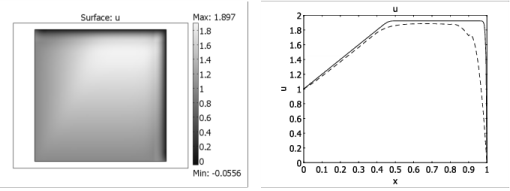
Figure 3-29 shows the effect of isotropic diffusion on Equation 3-5 with δid = 0.25. Although the solution is smooth, the comparison with the reference solution in the right plot reveals that the isotropic diffusion introduces far too much diffusion.

The streamline diffusion method in the COMSOL Multiphysics software is a consistent stabilization method. When applied to Equation 3-3, it recovers the streamline upwind Petrov-Galerkin (SUPG) method, but it can also recover functionality from the Galerkin least-squares (GLS) method. Both methods are described below. For theoretical details, see Ref. 1 and Ref. 2.

The theory underlying SUPG is a bit too complicated to describe here, but the resulting expressions can be shown to be closely related to upwinding schemes in finite difference and finite volume methods. SUPG can be shown to add a smaller amount of stability than isotropic diffusion (see Ref. 3), but while the accuracy of isotropic diffusion is at best O(h), the accuracy of SUPG can be shown to be at least O(hp+1/2) where p≥1 is the order of the basis functions.

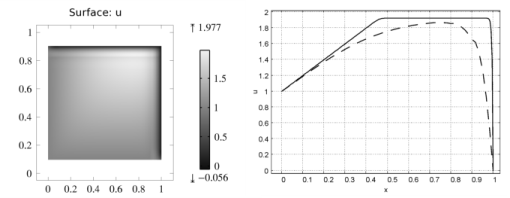
Figure 3-30 displays the effect of SUPG on the solution of Equation 3-5. The solution closely follows the reference solution away from the boundary layers, but at the boundary layers, oscillations occur. This is a typical behavior for streamline diffusion: the solution becomes smooth and exact in smooth regions but can contain local oscillations at sharp gradients.

Galerkin least-squares (GLS) is a more advanced version of SUPG, with which it shares many features. GLS, for example, is also a consistent method and has the same order of accuracy as SUPG. To understand the differences between GLS and SUPG, consider the following extended form of Equation 3-3:

where s is a production coefficient if s > 0 and an absorption coefficient if s < 0. If s ≠ 0, the numerical solution of Equation 3-7 is characterized by the Péclet number (see Equation 3-4) and the element Damköhler number:

The (unstabilized) Galerkin discretization becomes unstable if 2DaPe > 1 (Ref. 4), that is, if the production/absorption effects dominate over the viscous effects. GLS differs from SUPG in that GLS relaxes this requirement while SUPG does not.¹

Streamline diffusion introduces artificial diffusion in the streamline direction. This is often enough to obtain a smooth numerical solution if the exact solution of Equation 3-3 (or Equation 3-7) does not contain any discontinuities. At sharp gradients, however, undershoots and overshoots can occur in the numerical solutions (see Figure 3-30). Crosswind diffusion addresses these spurious oscillations by adding diffusion orthogonal to the streamline direction — that is, in the crosswind direction.

Crosswind diffusion methods are consistent, but they are also nonlinear. This means that the discrete equation system becomes nonlinear even if the original equation (Equation 3-3 or Equation 3-7) is linear, which can increase the computational cost.

The crosswind diffusion option adds a weak contribution as suggested in Ref. 5. For the scalar example here, the term reads

where gij is the covariant metric tensor. The coefficient νh is for Navier-Stokes systems a modified version of the Hughes-Mallet (HM) formulation of Ref. 6. In the scalar case, the modified HM formulation reduces effectively to the form suggested in Ref. 6. Additionally, Ref. 7 suggests to reduce νh for higher-order elements. The formulation in the COMSOL Multiphysics software multiplies νh with a factor

where N is the shape function order.

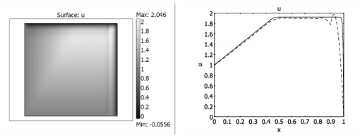
Figure 3-31 shows the example problem (Equation 3-5) solved using streamline diffusion and crosswind diffusion. Oscillations at the boundary layers are almost completely removed (compare with Figure 3-30), but it has been achieved by the introduction of some extra diffusion. In general, crosswind diffusion tries to smear out the boundary layer so that it becomes just wide enough to be resolved on the mesh (Figure 3-26). To obtain a sharper solution and remove the last oscillations, the mesh needs to be refined locally at the boundary layers.