The k-ε model is one of the most used turbulence models for industrial applications. This module includes the standard k-ε model (Ref. 1). The model introduces two additional transport equations and two dependent variables: the turbulent kinetic energy, k, and the turbulent dissipation rate, ε. The turbulent viscosity is modeled as

where Cμ is a model constant.

The transport equation for k reads:

The transport equation for ε reads:

The model constants in Equation 4-83, Equation 4-84, and Equation 4-86 are determined from experimental data (Ref. 1) and the values are listed in Table 4-3.

Equation 4-84 and Equation 4-86 cannot be implemented directly as written. There is, for example, nothing that prevents division by zero. The equations are instead implemented as suggested in Ref. 10. The implementation includes an upper limit on the mixing length, :

where δij is the Kronecker delta and Sij is the strain-rate tensor. The diagonal elements of the Reynolds stress tensor must be nonnegative, but calculating μT from Equation 4-83 does not guarantee this. To assert that

Combining equation Equation 4-88 with Equation 4-83 and the definition of the mixing length gives a limit on the mixing length scale:

Equivalently, combining Equation 4-89 with Equation 4-83 and Equation 4-87 gives:

This means there are two limitations on lmix: the realizability constraint and the imposed limit via Equation 4-87.

The effect of not applying a realizability constraint is typically excessive turbulence production. The effect is most clearly visible at stagnation points. To avoid such artifacts, the realizability constraint is always applied for the RANS models. More details can be found in Ref. 4, Ref. 5, and Ref. 6.

The k-ε turbulence model relies on several assumptions, the most important of which is that the Reynolds number is high enough. It is also important that the turbulence is in equilibrium in boundary layers, which means that production equals dissipation. These assumptions limit the accuracy of the model because they are not always true. It does not, for example, respond correctly to flows with adverse pressure gradients and can result in under-prediction of the spatial extent of recirculation zones (Ref. 1). Furthermore, in simulations of rotating flows, the model often shows poor agreement with experimental data (Ref. 2). In most cases, the limited accuracy is a fair tradeoff for the amount of computational resources saved compared to using more complicated turbulence models.

The flow close to a solid wall is for a turbulent flow very different from the free stream. This means that the assumptions used to derive the k-ε model are not valid close to walls. While it is possible to modify the k-ε model so that it describes the flow in wall regions (see The Low Reynolds Number k-ε Turbulence Model), this is not always desirable because of the very high resolution requirements that follow. Instead, analytical expressions are used to describe the flow near the walls. These expressions are known as wall functions.

When using wall functions in COMSOL Multiphysics, a theoretical lift-off from the physical wall is assumed as shown in Figure 4-7. Expressed in viscous units, the wall lift-off is defined as

The wall lift-off, δw, is defined as

where the friction velocity, uτ, is defined by

where in turn, κv, is the von Kárman constant (default value 0.41) and B is a constant that by default is set to 5.2. The two arguments for uτ are under some addition assumptions theoretically identical in the logarithmic layer (Ref. 1), but deviate in stagnation points and when the local Reynolds number becomes low. The definition of δw is such that it becomes h/2 when , but it can become larger when the lower limit for , 11.06, takes effect.

Wall functions give reasonable predictions as long as is lower than some upper limit that depends on the turbulent Reynolds number (Ref. 28). The upper limit is hardly ever lower than 50, and in many practical applications as high as a few hundred. Highest accuracy is obtained if is also everywhere larger than 25, which approximately corresponds to the beginning of the logarithmic layer. It can also be worthwhile to check that δw is small compared to the dimensions of the geometry, especially if for a significant fraction of the wall area.

The boundary conditions for the velocity is a no-penetration condition u ⋅ n = 0 and a shear stress condition

The turbulent kinetic energy is subject to a homogeneous Neumann condition n ⋅ ∇k = 0 and the boundary condition for ε reads:

See Ref. 10 and Ref. 11 for further details.

The physics interfaces Wall and Interior Wall have an option to apply wall roughness by modifying the wall functions. Cebeci (Ref. 21) suggested a model which adjusts the friction velocity for surface roughness,

is the roughness height in viscous units,

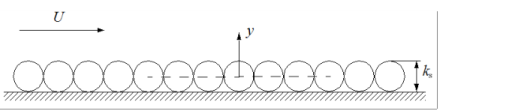
The roughness height, ks, is the peak-to-peak value of the surface variations and the wall is relocated to their mean level.

Hence, when Equation 4-92 is used the lift-off is modified according to,

where h+ is the height of the boundary mesh cell in viscous units. Cs is a parameter that depends on the shape and distribution of the roughness elements. When the turbulence parameters κν and B have the values 0.41 and 5.2, respectively, and Cs = 0.26, ks corresponds to the equivalent sand roughness height, kseq, as introduced by Nikuradse (Ref. 22). A few characteristic values of the equivalent sand roughness height are given in Table 4-4 below,

Use other values of the roughness parameter Cs and roughness height ks to specify generic surface roughnesses.

The default initial values for a stationary simulation are (Ref. 10),

where is the mixing length limit. For time-dependent simulations, the initial value for k is instead

The k-ε equations are derived under the assumption that the flow has a high enough Reynolds number. If this assumption is not fulfilled, both k and ε have very small magnitudes and behave chaotically in the manner that the relative values of k and ε can change by large amounts due to small changes in the flow field.

A time-dependent simulation of a turbulent flow can include a period when the flow is not fully turbulent. A typical example is the startup phase when for example an inlet velocity or a pressure difference is gradually increased. To sort out numerical fluctuations in k and ε during such periods, the default time-dependent solver for the k-ε model employs unscaled absolute tolerances for k and ε. The tolerances are set to

where Uscale and Lfact are input parameters available in the Advanced Settings section of the physics interface node. Their default values are 1 m/s and 0.035 respectively. lbb,min is the shortest side of the geometry bounding box. Equation 4-93 is closely related to the expressions for k and ε on inlet boundaries (see Equation 4-156).

The practical implication of Equation 4-93 is that variations in k and ε smaller than kscale and εscale respectively, are regarded as numerical noise.