Evaluating and plotting the acoustic pressure around radiating objects and sources is essential for the development of several acoustic devices. This is known as the spatial response or the radiation pattern. Application areas range from underwater acoustic transducers and loudspeakers, to determining the spatial sensitivity of microphone systems (for example, using reciprocity). Using the Exterior Field Calculation feature can help to reduce the computational domain while still being able to determine the pressure and thus the spatial response in the exterior field (near-field to far-field). The Radiation Pattern plots are specially designed for easy evaluation of the exterior field variables, that is, the acoustic exterior pressure and the exterior field sound pressure level.

In the radiation pattern plots, the exterior field variable (pressure or sound pressure level) is represented in a polar plot for a selected number of angles. Data is retrieved on an evaluation circle in 2D, 2D axial symmetry, or 3D. The angle interval and the number of angles can be manually specified. The evaluation circle origin, orientation, and radius can be specified as well as the reference direction. The evaluation circle can be visualized using a Preview Evaluation Plane functionality. There is also a built-in option to calculate the Beam Width of the plotted data. The data is stored in a table that can be plotted using the Table Graph option.

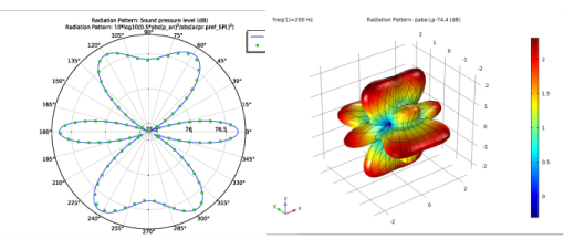
The 3D radiation pattern plots create a 3D polar plot (or bubble plot) where the data is evaluated on a sphere. Here, you can specify a separate expression for the surface color. In the 3D radiation pattern plots, the directivity can also be calculated by enabling the Compute directivity option. The result is given in a table and is calculated as the maximum power relative to the average power. The table comprises the maximal radiation direction (polar angles), the directivity, and the directivity given in dB (also known as the directivity index).

Variables defined by the Exterior Field Calculation feature like, for example, the pressure acpr.efc1.pext or sound pressure level acpr.efc1.Lp_pext are globally defined variables and can be directly evaluated in the Radiation Pattern plot and Directivity plot. The values plotted only make physical sense if they are evaluated outside of the Exterior Field Calculation boundary.

To visualize, for example, the sound pressure level inside of the Exterior Field Calculation boundary plot the expression: at2(x,y,acpr.Lp) in 2D, at2(r,z,acpr.Lp) in 2D axisymmetry, or at3(x,y,z,acpr.Lp) in 3D. The at2() and at3() operators ensure the variables are globally defined.

Another way of evaluating and depicting the exterior field is by using either the Grid 2D, the Grid 3D, the Parametrized Curve, or the Parametrized Surface data sets. Both types of data sets allow the evaluation of global quantities, like the exterior field variables, outside of the computational domain (outside of the mesh).

A dedicated Octave Band () plot exists to plot frequency response, transfer functions, transmission loss, and insertion loss curves. The plot has several built-in acoustics specific features like predefined weighting (Z, A, C, and User defined) as well as the possibility to plot the response in octaves, 1/3 octaves, 1/6 octaves, or as a continuous response.

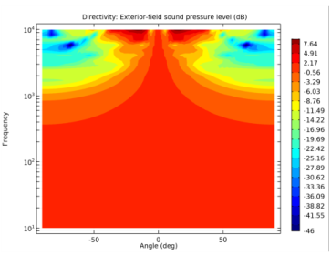
Another acoustics specific plot, especially used for loudspeakers, is the dedicated Directivity () plot. The plot allows audio engineers to depict the spatial response of a loudspeaker as function of both frequency and spatial angle in a contour-like plot. Representing the spatial response in this manner is a very common in the loudspeaker industry. Measured data is often also represented in the same manner. The plot includes many options to format the plot to achieve maximal insight into the modeled data, for example, linear and logarithmic frequency axis scaling options, easy switch of the x- and y-axis (frequency and polar angle axis), as well as options to normalize the data with respect to a given angle or the maximal value.