Octave Band
Use an Octave Band () plot to represent and plot a frequency response in frequency bands. An octave band plot corresponds to plotting the average or integrated value of, for example, the squared pressure over a given frequency band defined by the center frequency or midfrequency and the bandwidth. What the plot shows is a “white noise transfer function” of the system; that is, it assumes that the input is of the same nature as the output. The data input to an octave band plot is a frequency-domain solution; for example, it can be the acoustic pressure resulting from a Frequency Domain study or a parametric frequency sweep. To add this plot type, right-click a 1D Plot Group node and choose Octave Band from the More Plots menu.
Go to Common Results Node Settings for links to information about these sections: Data, Title, and Coloring and Style.
For examples that use an Octave Band plot, see Absorptive Muffler: Application Library path Acoustics_Module/Automotive/absorptive_muffler and The Brüel & Kjær 4134 Condenser Microphone: Application Library path Acoustics_Module/Electroacoustic_Transducers/bk_4134_microphone.
Selection
From the Geometric entity list, select the entity level (default: Point) for the evaluation of the octave band plot. Choose Global for a global evaluation. If you select line, boundary, or domain, the quantity will be averaged. You can use those entity levels to plot the response as the average over the outlet of a system, for example. Then, except for Global, use the selection tools to select geometric entities on that level for the evaluation.
y-Axis Data
In the Expression field, enter an expression for the input to the octave band plot. Click the Replace Expression () or Insert Expression () button to select predefined expressions based on the physics of the model. If you want to add a description of the expression for the plot title, select the Description check box and enter a description in the text field below.
From the Expression type list, choose one of the following types:
Amplitude (the default), to compute the octave plot treating the expression as an amplitude prms. The input is the value p (it is generally a complex-valued variable). It is in turn used to calculate the rms pressure prms, which defines the level L:
In the Amplitude reference field, enter a value of expression for an amplitude reference pref. Click the Replace Expression () to pick an amplitude reference from a list of predefined expressions.
Power, to compute the octave plot treating the expression as a power P, which defines the level L:
In the Power reference field, enter a value of expression for a power reference Pref. Click Replace Expression () to pick a power reference from a list of predefined expressions.
Transfer function, to compute the octave plot treating the expression as a transfer function H (generally, a complex-valued variable), which defines the level L:
In the Level reference field, enter a value of expression for a level reference Lref. Click Replace Expression () to pick a level reference from a list of predefined expressions.
Underneath those settings, the mathematical formula used for each expression type is displayed.
Outside the frequency range, the signal is assumed to be zero and no extrapolation is done.
Plot
You can choose one of the following styles of the octave band plot from the Style list:
Continuous, to plot a continuous response
Octave bands (the default), to plot the response using octave bands.
1/3 octave bands, to plot the response using 1/3 octave bands.
1/6 octave bands, to plot the response using 1/6 octave bands.
For the Octave band, 1/3 octave band, and 1/6 octave band styles, the Use in-band data only check box is selected by default to use an integral that is evaluated as an average only based on data points inside the octave or 1/3 octave bands.
You can use some predefined weighting or a user-defined weighting of the frequency data. The frequency weighting is used in acoustics to shape the response to match the characteristics of the human ear.
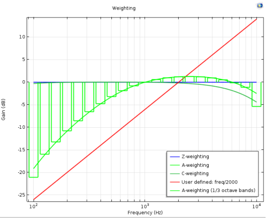
The predefined weightings are defined in IEC 61672-1. See IEC 61672-1 Electroacoustics - Sound level meters - Part 1: Specifications for details.
From the Weighting list, select:
Z-weighted (flat) (the default), to use a zero weighting; that is, a flat weighting.
A-weighted, to use a weighting that mimics the loudness perceived by the human ear.
C-weighted, to use a C-weighting, which is an alternative standardized weighting that is in use within the acoustics community.
Expression, to enter a user-defined value or expression for the weighting in the Expression field. The expression defines the gain as a function of the frequency. The gain given in dB is then given as 20·log10(expression). Use the frequency variable freq for user-defined expressions.
The following COMSOL Multiphysics plot shows the different weighting types as gain (dB) versus frequency (Hz):
Figure 21-7: The plot shows Z-weighting (blue), A-weighting (light green), C-weighting (dark green), and a user-defined weighting (red). The 1/3 octave bands (light green) also show A-weighting.
Legends
Select the Show legends check box to display the plotted expressions to the right of the plot. In plots where each line represents a certain time value, eigenvalue, or parameter value, these values are also displayed.
When Automatic is selected from the Legends list (the default), select or clear the Description and Expression check boxes to control what to include in the automatic legends (by default it includes the description only). If Manual is selected from the Legends list, enter your own legend text into the table.