Release
Use the Release node to release rays within domains based on arbitrary expressions or based on the positions of the mesh elements.
release times
This section is only available when the Allow multiple release times check box has been selected in the physics interface Advanced Settings section. Enter Release times (SI unit: s) or click the Range button () to select and define a range of specific times. At each release time, rays are released with initial position and ray direction vector as defined next.
Initial Position
Select an Initial position: Density (the default) or Mesh based.
Density
For Density enter a value for the Number of rays per release N (dimensionless). The default is 100. Then enter a value or expression for the Density proportional to ρ (dimensionless). The default is 1.
The Density proportional to ρ can be an expression rather than a number; the resulting ray distribution approximately has a number density that is proportional to this expression. The resulting distribution looks a bit random, and it depends on the order in which the mesh elements are numbered. The distribution is probably not exactly the same in different COMSOL Multiphysics versions, but the total number of rays released is always N.
The Density proportional to expression must be strictly positive.
Advanced Options for Density-Based Release
The following options can be adjusted to make the number density of rays more closely conform to the Density proportional to expression.
Select a Release distribution accuracy order between 1 and 5 (the default is 5), which determines the integration order that is used when computing the number of rays to release within each mesh element. The higher the accuracy order, the more accurately rays will be distributed among the mesh elements.
The Position refinement factor (default 0) must be a nonnegative integer. When the refinement factor is 0, each ray is always assigned a unique position, but the density is taken as a uniform value over each mesh element. If the refinement factor is a positive integer, the distribution of rays within each mesh element is weighted according to the density, but it is possible for some rays to occupy the same initial position. Further increasing the Position refinement factor increases the number of evaluation points within each mesh element to reduce the probability of multiple rays occupying the same initial position.
Mesh Based
For Mesh based the rays are released from a set of positions determined by a selection of geometric entities (of arbitrary dimension) in the mesh. Given a Refinement factor between 1 and 5, the centers of the refined mesh elements are used. Thus, the number of positions per mesh element is refine^dim, except for pyramids, where it is (4*refine2-1)*refine/3.
Ray Direction Vector
Select an option from the Ray direction vector list: Expression (the default), Spherical, Hemispherical, Conical, or Lambertian (3D only).
For Expression a single ray is released in the specified direction. Enter coordinates for the Ray direction vector L0 (dimensionless) based on space dimension.
For Spherical a number of rays are released at each point, sampled from a spherical distribution in wave vector space. Enter the Number of rays in wave vector space Nw (dimensionless). The default is 50.
For Hemispherical a number of rays are released at each point, sampled from a hemispherical distribution in wave vector space. Enter the Number of rays in wave vector space Nw (dimensionless). The default is 50. Then enter coordinates for the Hemisphere axis r based on space dimension.
For Conical a number of rays are released at each point, sampled from a conical distribution in wave vector space. Enter the Number of rays in wave vector space Nw (dimensionless). The default is 50. Then enter coordinates for the Cone axis r based on space dimension. Then enter the Cone angle α (SI unit: rad). The default is π/3 radians.
The Lambertian option is only available in 3D. A number of rays are released at each point, sampled from a hemisphere in wave vector space with probability density based on the cosine law. Enter the Number of rays in wave vector space Nw (dimensionless). The default is 50. Then enter coordinates for the Hemisphere axis r based on space dimension.
If Conical is selected, select an option from the Conical distribution list: Uniform density (the default), Specify polar and azimuthal distributions, Hexapolar, Marginal rays only, or Marginal and axial rays only.
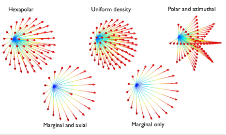
For Uniform density rays are released with polar angles from 0 to the specified cone angle. The rays are distributed in wave vector space so that each ray subtends approximately the same solid angle.
For Specify polar and azimuthal distributions specify the Number of polar angles Nθ (dimensionless) and the Number of azimuthal angles Nϕ (dimensionless). Rays are released at uniformly distributed polar angles from 0 to the specified cone angle. A single axial ray (θ = 0) is also released. For each value of the polar angle, rays are released at uniformly distributed azimuthal angles from 0 to 2π. Unlike other options for specifying the conical distribution, it is not necessary to directly specify the Number of rays in wave vector space Nw (dimensionless), which is instead derived from the relation Nw = Nθ × Nϕ + 1.
For Hexapolar specify the Number of polar angles Nθ (dimensionless). In this distribution, for each release point, one ray will be released along the cone axis. Six rays are released at an angle α/Nθ from the cone axis, then 12 rays at an angle of 2α/Nθ, and so on. The total number of ray directions in the distribution is Nw = 3Nθ(Nθ + 1) + 1.
For Marginal rays only the rays are all released at an angle α with respect to the cone axis. The rays are released at uniformly distributed azimuthal angles from 0 to 2π.
For Marginal and axial rays only the rays are all released at an angle α with respect to the cone axis, except for one ray which is released along the cone axis. The marginal rays are released at uniformly distributed azimuthal angles from 0 to 2π.
Figure 8-1: Comparison of the four available cone-based release distributions.
For Spherical, Hemispherical, Conical, and Lambertian, select an option from the Sampling from Distribution list: Deterministic (the default) or Random. If Deterministic is selected, the initial ray direction vectors are computed using an algorithm that seeks to distribute the rays as evenly as possible in wave vector space. This algorithm will give the same initial ray directions whenever the study is run. If Random is selected, the initial direction of each ray is sampled from a probability distribution in wave vector space using pseudorandom numbers. The result may be the same when rerunning the study multiple times on the same computer, but the solution is likely to be different on different architectures.
For Expression it is also possible to initialize the ray direction vector either in the global coordinate system or in a coordinate system that moves with the same velocity as the background medium. Select an option from the Initial wave vector specification list: With respect to fluid (the default) or With respect to coordinate system.
For With respect to fluid the initial wave vector is computed with respect to a coordinate system that moves at the background velocity, so the initial ray direction might not be parallel to the vector entered in the Ray direction vector text field if the medium is moving.
For With respect to coordinate system the initial ray direction is parallel to the vector entered in the Ray direction vector text field as long as a ray could reasonably propagate in that direction. For example, rays cannot be released in certain directions if the background fluid is moving with a supersonic velocity.
Initial Ray Frequency
This section is available when the Allow frequency distributions at release features check box is selected under the physics interface Ray Release and Propagation section.
Select a Distribution function: None (the default), Normal, Lognormal, Uniform, or List of values.
When None is selected, enter an initial value f0 (SI unit: Hz). The default value is 1000 Hz.
Select Normal to create a normal distribution function, Lognormal to create a log-normal distribution function, or Uniform to create a uniform distribution function. For any of these selections, the Number of values sets the number of points in the distribution function. Enter a user-defined Mean (default 1000 Hz) and Standard deviation (default 100 Hz). Select List of values to enter a list of distinct frequency values.
Initial Phase
This section is available when the Compute phase check box is selected under the physics interface Intensity Computation section. Enter an Initial phase Ψ0 (SI unit: rad). The default value is 0.
Initial Intensity
This section is available when the ray intensity is solved for in the model and Expression is selected as the Ray direction vector. Enter a value for the Initial intensity I0 (SI unit: W/m2). The default is 1000 W/m2.
Initial Radii of Curvature
This section is available when the ray intensity is solved for in the model and Expression is selected as the Ray direction vector. Select a Wavefront shape. In 3D the available options are Plane wave (the default), Spherical wave, and Ellipsoid. In 2D the available options are Plane wave (the default) and Cylindrical wave.
For an idealized plane wave the radii of curvature would be infinite. However, because the algorithm used to compute intensity requires finite values, when Plane wave is selected the initial radii of curvature are instead given an initial value that is 108 times greater than the characteristic size of the geometry.
For a Spherical wave or Cylindrical wave, enter the Initial radius of curvature r0 (SI unit: m).
For an Ellipsoid, enter the Initial radius of curvature, 1 r1,0 (SI unit: m) and the Initial radius of curvature, 2 r2,0 (SI unit: m). Also enter the Initial principal curvature direction, 1 e1,0 (dimensionless).
For spherical and cylindrical waves the Initial radius of curvature must be nonzero. To release a ray such that the initial wavefront radius of curvature is zero, instead select a different option such as Conical from the Ray direction vector list.
Total Source Power
This section is available:
when Spherical, Hemispherical, or Conical is selected as the Ray direction vector.
Enter a Total source power Psrc (SI unit: W). The default is 1 W. In 2D, instead enter the Total source power per unit thickness Psrc (SI unit: W/m). The default is 1 W/m.
Initial Value of Auxiliary Dependent Variables
This section is available if an Auxiliary Dependent Variable has been added to the model.
For each of the Auxiliary Dependent Variable nodes added to the model, select a Distribution function for the initial value of the auxiliary dependent variables and whether the initial value of the auxiliary dependent variables should be a scalar value or sampled from a distribution function.
The number of rays simulated can increase substantially and the following options are available for each Auxiliary Dependent Variable added to the model.
When None is selected, enter an initial value. The symbol for the initial value is the auxiliary variable name followed by a subscript 0, so for the default name rp the initial value has symbol rp0.
For the initial value of the auxiliary dependent variables, select Normal to create a normal distribution function, Lognormal to create a log-normal distribution function, or Uniform to create a uniform distribution function. For any selection, the Number of values sets the number of points in the distribution function. Enter a user-defined Mean (default 0) and Standard deviation (default 1). Select List of values to enter a set of numerical values directly.
By default auxiliary dependent variables are initialized after all other degrees of freedom. Select the Initialize before wave vector check box to compute the initial value of the auxiliary dependent variable immediately after computing the initial wave vectors of the rays. By selecting this check box it is possible to define the initial ray direction as a function of the auxiliary dependent variables.