The Electromagnetic Waves, Frequency Domain Interface

The interface (

), found under the branch (

) when adding a physics interface, is used to solve for time-harmonic electromagnetic field distributions.

For this physics interface, the maximum mesh element size should be limited to a fraction of the wavelength. The domain size that can be simulated thus scales with the amount of available computer memory and the wavelength. The physics interface supports the study types Frequency Domain, Wavelength Domain, Eigenfrequency, Mode Analysis, and Boundary Mode Analysis. The Frequency Domain and Wavelength Domain study types are used for source driven simulations for a single frequency/wavelength or a sequence of frequencies/wavelengths. The Eigenfrequency study type is used to find resonance frequencies and their associated eigenmodes in resonant cavities.

This physics interface solves the time-harmonic wave equation for the electric field.

When this physics interface is added, these default nodes are also added to the — , , and . Then, from the toolbar, add other nodes that implement, for example, boundary conditions. You can also right-click to select physics features from the context menu.

The Mode analysis study type is applicable only for 2D and 2D axisymmetric cross-sections of waveguides and transmission lines where it is used to find allowed propagating modes. Boundary mode analysis is used for the same purpose in 2D, 2D axisymmetry, and 3D and applies to boundaries representing waveguide ports.

The is the default physics interface name.

The is used primarily as a scope prefix for variables defined by the physics interface. Refer to such physics interface variables in expressions using the pattern <name>.<variable_name>. In order to distinguish between variables belonging to different physics interfaces, the name string must be unique. Only letters, numbers, and underscores (_) are permitted in the field. The first character must be a letter.

The default (for the first physics interface in the model) is ewfd.

From the list, select whether to solve for the (the default) or the .

For select a — (the default), , or.

Enter the component expressions for the Eb (SI unit: V/m). The entered expressions must be differentiable.

	Notice that expressions including coupling operators are not differentiable and cannot be used as background fields.

The Gaussian beam background field is a solution to the paraxial wave equation, which is an approximation to the Helmholtz equation solved for by the interface. The approximation is valid for Gaussian beams that have a beam radius that is much larger than the wavelength. Since the paraxial Gaussian beam background field is an approximation to the Helmholtz equation, for tightly focused beams, you can get a nonzero scattered field solution, even if you do not have any scatterers. For more information about the Gaussian beam theory, see Gaussian Beams as Background Fields.

•

Enter a k (SI unit: rad/m). The default is ewfd.k0 rad/m. The wave number must evaluate to a value that is the same for all the domains the scattered field is applied to. Setting the k to a positive value, means that the wave is propagating in the positive x-, y-, or z-axis direction, whereas setting the k to a negative value means that the wave is propagating in the negative x-, y-, or z-axis direction.

The initial background wave is predefined as E0 = exp(−jkxx)z. This field is transformed by three successive rotations along the roll, pitch, and yaw angles, in that order. For a graphic representation of the initial background field and the definition of the three rotations, c.f. Figure 3-1 below.

•

Enter a (SI unit: rad), which is a right-handed rotation with respect to the +x-direction. The default is 0 rad, corresponding to polarization along the +z-direction.

•

Enter a (SI unit: rad), which is a right-handed rotation with respect to the +y-direction. The default is 0 rad, corresponding to the initial direction of propagation pointing in the +x-direction.

•

Enter a k (SI unit: rad/m). The default is ewfd.k0 rad/m. The wave number must evaluate to a value that is the same for the domains the scattered field is applied to.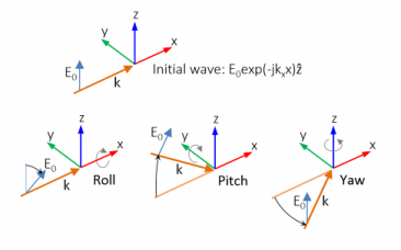

Figure 3-1: Schematic of the directions for the wave vector k, the electric field E0, and the roll, pitch and yaw rotations. The top image represents an initial wave propagating in the x direction with a polarization along the z direction.

This section is available for 2D and 2D axisymmetric components.

Select the — , , or . Select:

•

to solve for the electric field vector component perpendicular to the modeling plane, assuming that there is no electric field in the plane.

•

to solve for the electric field vector components in the modeling plane assuming that there is no electric field perpendicular to the plane.

This section is available for 2D and 2D axisymmetric components, when solving for or.

For 2D components, assign a wave vector component to the field. For 2D axisymmetric components, assign an integer constant or an integer parameter expression to the field.

Select the check box to use a physics-controlled mesh for the electromagnetic problem. When selected, this invokes a parameter for the maximum mesh element size in free space. The physics-controlled mesh automatically scales the maximum mesh element size as the wavelength changes in different dielectric and magnetic regions. If the model is configured by any periodic conditions, identical meshes are generated on each pair of periodic boundaries. Perfectly matched layers are built with a structured mesh, specifically, a swept mesh in 3D and a mapped mesh in 2D.

When is selected, choose one of the three options for the — (the default), , or . For the option , enter a suitable . For example, 1/5 of the vacuum wavelength or smaller. When is selected, enter the highest frequency intended to be used during the simulation. The maximum mesh element size in free space is 1/5 of the vacuum wavelength for the entered frequency. For the option, enter the smallest vacuum wavelength intended to be used during the simulation. The maximum mesh element size in free space is 1/5 of the entered wavelength.

When is selected, the outer boundaries of lossy media domains are meshed with a maximum mesh element size in free space given by the minimum value of half a skin depth and 1/5 of the vacuum wavelength.

The maximum mesh element size in dielectric media is that in free space divided by the square root of the product of the relative permittivity and permeability.

Select the check box to switch on the port sweep. When selected, this invokes a parametric sweep over the ports in addition to the automatically generated frequency/wavelength sweep. The generated lumped parameters are in the form of an S-parameter matrix.

For enter a to assign a specific name to the parameter that controls the port number solved for during the sweep. Before making the port sweep, the parameter must also have been added to the list of parameters in the section of the node under the node.

For this physics interface, the S-parameters are subject to . Click to locate the file, or enter a file name and path. Select an : , , or .

Enter a , Zref (SI unit: Ω). The default is 50 Ω.

The dependent variables (field variables) are for the E and its components (in the fields). The name can be changed but the names of fields and dependent variables must be unique within a model.