Release
Use the Release node to release rays within domains based on arbitrary expressions or based on the positions of the mesh elements.
release times
Enter Release times (SI unit: s) or click the Range button () to select and define a range of specific times. At each release time, rays are released with initial position and ray direction vector as defined next.
This section is only available when the Allow multiple release times property is active. This can be found in the Advanced section of the physics interface settings when Advanced Physics Options are shown in the Model Builder.
Initial Position
Select an Initial positionDensity (the default) or Mesh based.
Density
For Density enter a value for the Number of rays per release N and the Density proportional to ρ. Both are dimensionless numbers.
The Density proportional to ρ is an expression — the resulting ray distribution approximately has a density that is proportional to this expression. The resulting distribution looks a bit random, and it depends on the order in which the mesh elements are numbered. The distribution is probably not exactly the same in different COMSOL Multiphysics versions, but the total number of rays released is always N.
The Density proportional to expression must be strictly positive.
Select a Release distribution accuracy order between 1 and 5 (the default is 5), which determines the integration order that is used when computing the number of rays to release within each mesh element. The higher the accuracy order, the more accurately rays will be distributed among the mesh elements.
The Position refinement factor (default 0) must be a nonnegative integer. When the refinement factor is 0, each ray is always assigned a unique position, but the density is taken as a uniform value over each mesh element. If the refinement factor is a positive integer, the distribution of rays within each mesh element is weighted according to the density, but it is possible for some rays to occupy the same initial position. Further increasing the Position refinement factor increases the number of evaluation points within each mesh element to reduce the probability of multiple rays occupying the same initial position.
Mesh Based
For Mesh based the rays are released from a set of positions determined by a selection of geometric entities (of arbitrary dimension) in the mesh. Given a Refinement factor between 1 and 5, the centers of the refined mesh elements are used. Thus, the number of positions per mesh element is refine^dim, except for pyramids, where it is (4*refine2-1)*refine/3.
Ray Direction Vector
Select an option from the Ray direction vector list — Expression (the default), Spherical, Hemispherical, Conical, or Lambertian (3D only).
For Expression a single ray is released in the specified direction. Enter coordinates for the Ray direction vector L0 (dimensionless) based on space dimension.
For Spherical a number of rays are released at each point, sampled from a spherical distribution in wave vector space. Enter the Number of rays in wave vector space Nw (dimensionless). The default is 50.
For Hemispherical a number of rays are released at each point, sampled from a hemispherical distribution in wave vector space. Enter the Number of rays in wave vector space Nw (dimensionless). The default is 50. Then enter coordinates for the Hemisphere axis r based on space dimension.
For Conical a number of rays are released at each point, sampled from a conical distribution in wave vector space. Enter the Number of rays in wave vector space Nw (dimensionless). The default is 50. Then enter coordinates for the Cone axis r based on space dimension. Then enter the Cone angle α (SI unit: rad). The default is π/3 radians.
The Lambertian option is only available in 3D. Anumber of rays are released at each point, sampled from a hemisphere in wave vector space with probability density based on the cosine law. Enter the Number of rays in wave vector space Nw (dimensionless). The default is 50. Then enter coordinates for the Hemisphere axis r based on space dimension.
If Conical is selected, select an option from the Conical distribution list — Uniform density (the default), Specify polar and azimuthal distributions, Marginal rays only, or Marginal and axial rays only.
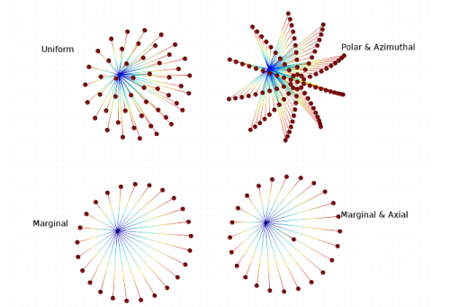
For Specify polar and azimuthal distributions specify the Number of polar angles Nφ (dimensionless) and the Number of azimuthal angles Nθ (dimensionless). Rays are released at uniformly distributed polar angles from 0 to the specified cone angle. A single axial ray (φ = 0) is also released. For each value of the polar angle, rays are released at uniformly distributed azimuthal angles from 0 to 2π. Unlike other options for specifying the conical distribution, it is not necessary to directly specify the Number of rays in wave vector space Nw (dimensionless), which is instead derived from the relation .
For Marginal rays only the rays are all released at an angle α with respect to the cone axis. The rays are released at uniformly distributed azimuthal angles from 0 to 2π.
For Marginal and axial rays only the rays are all released at an angle α with respect to the cone axis, except for one ray which is released along the cone axis. The marginal rays are released at uniformly distributed azimuthal angles from 0 to 2π.
Figure 3-1: Comparison of the four available cone-based release distributions.
For Spherical, Hemispherical, Conical, and Lambertian, select an option from the Sampling from Distribution list — Deterministic (the default) or Random. If Deterministic is selected, the initial ray direction vectors are computed using an algorithm that seeks to distribute the rays as evenly as possible in wave vector space. This algorithm will give the same initial ray directions whenever the study is run. If Random is selected, the initial direction of each ray is sampled from a probability distribution in wave vector space using pseudorandom numbers. The result may be the same when rerunning the study multiple times on the same computer, but the solution is likely to be different on different architectures.
Initial Ray Frequency
This section is available when the Allow frequency distributions at release features check box is selected under the physics interface Ray Release and Propagation section.
Select a Distribution functionNone (the default), Normal, Lognormal, Uniform, or List of values.
When None is selected, enter an initial value ν0. The default value is 4.54 × 1014 Hz.
Select Normal to create a normal distribution function, Lognormal to create a log-normal distribution function, or Uniform to create a uniform distribution function. For any of these selections, the Number of values sets the number of points in the distribution function. Enter a user-defined Mean (default 4.54 × 1014 Hz) and Standard deviation (default 1014 Hz). Select List of values to enter a list of distinct frequency values.
Initial Phase
This section is available when the Compute phase check box is selected under the physics interface Intensity Computation section. Enter an Initial phase Ψ0 (SI unit: rad). The default value is 0.
Initial Intensity
This section is available when:
the Intensity computation is set to Compute intensity, Compute intensity and power, Compute intensity in graded media, or Compute intensity and power in graded media in the physics interface Intensity Computation section, and
Expression is selected as the Ray direction vector.
Enter a value for the Initial intensity I0 (SI unit: W/m2). The default is 1000 W/m2.
Initial Radii of Curvature
This section is available when:
the Intensity computation is set to Compute intensity, Compute intensity and power, Compute intensity in graded media, or Compute intensity and power in graded media in the physics interface Intensity Computation section, and
Expression is selected as the Ray direction vector.
Select a Wavefront shape. In 3D the available options are Plane wave (the default), Spherical wave, and Ellipsoid. In 2D the available options are Plane wave (the default) and Cylindrical wave.
For an idealized plane wave the radii of curvature would be infinite. However, because the algorithm used to compute intensity requires finite values, when Plane wave is selected the initial radii of curvature are instead given an initial value that is 108 times greater than the characteristic size of the geometry.
For a Spherical wave or Cylindrical wave, enter the Initial radius of curvature r0 (SI unit: m).
For an Ellipsoid, enter the Initial radius of curvature, 1 r1,0 (SI unit: m) and the Initial radius of curvature, 2 r2,0 (SI unit: m). Also enter the Initial principal curvature direction, 1 e1,0 (dimensionless).
Initial Polarization
This section is available when the Intensity computation is set to Compute intensity, Compute intensity and power, Compute intensity in graded media, or Compute intensity and power in graded media under the physics interface Intensity Computation section.
Select an Initial polarization typeUnpolarized (the default), Fully polarized, or Partially polarized.
Select an Initial polarizationAlong principal curvature direction (the default) or User defined.
For Fully polarized and Partially polarized rays in 3D enter an Initial polarization parallel to reference direction a1,0 (dimensionless), Initial polarization perpendicular to reference direction a2,0 (dimensionless), and Initial phase difference δ0 (SI unit: rad).
For Fully polarized and Partially polarized rays in 2D enter an Initial polarization, in plane axy,1 (dimensionless), Initial polarization, out of plane az,0 (dimensionless), and Initial phase difference δ0 (SI unit: rad).
For User defined also enter an Initial polarization reference direction u (dimensionless).
For Partially polarized, also enter an Initial degree of polarization P0 (dimensionless).
Total Source Power
This section is available:
when the Intensity computation is set to Compute intensity or Compute intensity in graded media under the physics interface Intensity Computation section, and
when Spherical, Hemispherical, or Conical is selected as the Ray direction vector.
It is also available when the Intensity computation is Compute intensity and power or Compute intensity and power in graded media under the physics interface Intensity Computation section, and any choice of Ray direction vector displays this section.
Select an option from the Intensity initialization list. By default Uniform distribution is selected. If any Photometric Data Import nodes have been added to the model then they can also be selected from the list.
If Uniform distribution is selected, enter a Total source power Psrc (SI unit: W). The default is 1 W. In 2D, instead enter the Total source power per unit thickness Psrc (SI unit: W/m). The default is 1 W/m. If any Photometric Data Import feature is selected from the list, the source power is instead obtained directly from the imported photometric data (IES) file. Enter values or expressions for the components of the Photometric horizontal ph (dimensionless) and Photometric zero pz (dimensionless). By default these vectors point in the positive x- and z-axes, respectively.
The relationship between the photometric horizontal, photometric vertical, and ray direction vector, and its effect on the initial ray intensity, is explained in ANSI/IESNA LM-63-02 (R2008), IESNA Standard file format for the electronic transfer of photometric data and related information, Illuminating Engineering Society (2002).
Currently the Photometric Data Import feature does not support the options TILT=INCLUDE or TILT=<FILENAME> that are included in some IES files. Only TILT=NONE is allowed.
Initial Value of Auxiliary Dependent Variables
This section is available if an Auxiliary Dependent Variable has been added to the model.
For each of the Auxiliary Dependent Variable nodes added to the model, select a Distribution function for the initial value of the auxiliary dependent variables and whether the initial value of the auxiliary dependent variables should be a scalar value or sampled from a distribution function.
The number of rays simulated can increase substantially and the following options are available for each Auxiliary Dependent Variable added to the model.
When None is selected, enter an initial value. The symbol for the initial value is the auxiliary variable name followed by a subscript 0, so for the default name rp the initial value has symbol rp0.
For the initial value of the auxiliary dependent variables, select Normal to create a normal distribution function, Lognormal to create a log-normal distribution function, or Uniform to create a uniform distribution function. For any selection, the Number of values sets the number of points in the distribution function. Enter a user-defined Mean (default 0) and Standard deviation (default 1). Select List of values to enter a set of numerical values directly.
By default auxiliary dependent variables are initialized after all other degrees of freedom. Select the Initialize before wave vector check box to compute the initial value of the auxiliary dependent variable immediately after computing the initial wave vectors of the rays. By selecting this check box it is possible to define the initial ray direction as a function of the auxiliary dependent variables.