Postprocessing Tools
The Ray Optics Module includes several tools for visualizing and analyzing ray trajectories. The following sections describe the dedicated postprocessing tools for the Geometrical Optics interface.
Ray Trajectories Plot
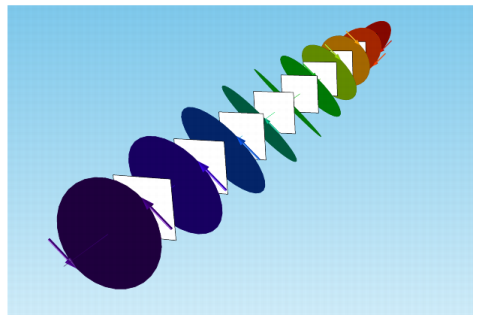
The Ray Trajectories plot can be added to a 2D or 3D plot group. By default, the trajectory of each ray is plotted as a line. As shown in Figure 2-2, it is also possible to apply color expressions and deformations to Ray Trajectories plots.
When the ray intensity is computed, built-in variables for the semi-major and semi-minor axes of the polarization ellipse are declared. For a physics interface with name gop, the semi-major axis has components gop.pax, gop.pay, and gop.paz. The semi-minor axis has components gop.pbx, gop.pby, and gop.pbz.
Figure 2-11: Polarization ellipses for a circularly polarized ray passing through a series of linear wave retarders with parallel fast axes.
Ray Plot
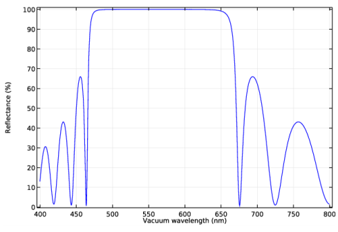
The Ray plot can be added to 1D plot groups. The Ray plot can be used to plot any ray property over time. Built-in data series operations allow quantities like the sum or maximum value of an expression over all rays to be computed easily.
Alternatively, two ray properties can be plotted against each other at a specific time. This can be used, for example, to compare ray intensity versus free-space wavelength, or to view optical path length as a function of radial position in a beam.
Figure 2-12: Reflectance of a distributed Bragg reflector with 21 dielectric layers is plotted as a function of free-space wavelength.
Interference Pattern Plot
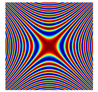
The pattern of fringes resulting from the interference of two or more rays can be plotted using the dedicated Interference Pattern plot. The Interference Pattern plot is available in 2D plot groups and requires a Cut Plane data set pointing to a Ray data set. The interference pattern is then plotted using the locations and properties of rays as they intersect the cut plane.
For the resulting interference pattern to be physically meaningful, it must be plotted over a region with a length scale that is much smaller than the principal radii of curvature of the incident wavefronts. This is equivalent to the assumption that the wavefront associated with each ray subtends a very small solid angle, and is necessary due to the approximation used to compute the incident intensity.
Figure 2-13: Interference pattern resulting from two parallel rays with elliptical wavefronts of different principal radii of curvature.
Poincaré Maps and Phase Portraits
A Poincaré Map can be used to plot the intersection points of rays with a plane. To use the Poincaré Map, a Cut Plane data set must first be defined.
By placing the Cut Plane data set at the image plane of an optical system, it is possible to use the Poincaré Map to create spot diagrams in order to evaluate the performance of the optical system.
A Phase Portrait can be used to plot the positions of rays in an arbitrarily defined phase space. For example, it is possible to plot rays in a 2D space in which one coordinate represents the optical path length and the other coordinate represents intensity.