|
|
|
|
m-1
|
||||
|
kg/m3
|
|||
|
m3/kg
|
|||
|
m2/d
|
|||
|
|
d-1
|
||
|
|
d-1
|
||
|
1
|
|
2
|
In the Select Physics tree, select Fluid Flow>Porous Media and Subsurface Flow>Richards’ Equation (dl).
|
|
3
|
Click Add.
|
|
4
|
In the Select Physics tree, select Chemical Species Transport>Transport of Diluted Species in Porous Media (tds).
|
|
5
|
Click Add.
|
|
6
|
Click Study.
|
|
7
|
|
8
|
Click Done.
|
|
1
|
|
2
|
|
3
|
|
4
|
Browse to the model’s Application Libraries folder and double-click the file sorbing_solute_parameters.txt.
|
|
1
|
|
2
|
|
3
|
|
4
|
|
5
|
|
6
|
|
7
|
|
1
|
|
2
|
|
3
|
|
4
|
|
5
|
|
6
|
|
7
|
|
1
|
|
2
|
|
3
|
|
4
|
|
5
|
|
1
|
|
3
|
|
4
|
|
1
|
In the Model Builder window, under Component 1 (comp1)>Richards’ Equation (dl) click Richards’ Equation Model 1.
|
|
2
|
|
3
|
|
4
|
Locate the Matrix Properties section. From the Permeability model list, choose Hydraulic conductivity.
|
|
5
|
|
6
|
|
7
|
|
8
|
Locate the Storage Model section. From the Storage list, choose User defined. In the S text field, type Ss_1.
|
|
9
|
|
10
|
|
1
|
Right-click Component 1 (comp1)>Richards’ Equation (dl)>Richards’ Equation Model 1 and choose Duplicate.
|
|
3
|
|
4
|
|
5
|
|
6
|
|
7
|
|
8
|
|
9
|
|
1
|
In the Model Builder window, under Component 1 (comp1)>Richards’ Equation (dl) click Initial Values 1.
|
|
2
|
|
3
|
|
4
|
|
1
|
|
3
|
|
4
|
|
1
|
|
3
|
|
4
|
|
1
|
|
2
|
|
4
|
|
5
|
|
6
|
|
1
|
|
2
|
|
3
|
|
1
|
In the Model Builder window, under Component 1 (comp1) click Transport of Diluted Species in Porous Media (tds).
|
|
2
|
In the Settings window for Transport of Diluted Species in Porous Media, locate the Transport Mechanisms section.
|
|
3
|
|
1
|
|
2
|
|
3
|
|
4
|
|
5
|
Locate the Matrix Properties section. From the εp list, choose User defined. In the associated text field, type dl.thetas.
|
|
6
|
|
7
|
|
8
|
|
9
|
|
10
|
|
11
|
|
12
|
|
13
|
|
14
|
|
15
|
In the α table, enter the following settings:
|
|
1
|
|
2
|
|
3
|
|
4
|
|
1
|
|
2
|
|
3
|
|
4
|
|
1
|
|
1
|
|
3
|
|
4
|
|
5
|
|
1
|
|
2
|
|
3
|
|
1
|
|
2
|
|
3
|
|
4
|
|
6
|
|
7
|
|
9
|
|
10
|
|
1
|
|
2
|
|
3
|
|
4
|
|
1
|
|
2
|
|
3
|
|
1
|
|
2
|
|
3
|
|
1
|
|
2
|
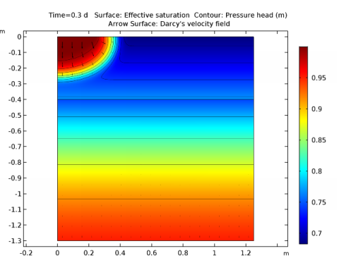
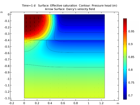
In the Settings window for Surface, click Replace Expression in the upper-right corner of the Expression section. From the menu, choose Model>Component 1>Richards’ Equation>dl.Se - Effective saturation.
|
|
3
|
|
4
|
|
1
|
|
2
|
In the Settings window for Contour, click Replace Expression in the upper-right corner of the Expression section. From the menu, choose Model>Component 1>Richards’ Equation>dl.Hp - Pressure head.
|
|
3
|
|
4
|
|
5
|
|
6
|
|
7
|
|
1
|
|
2
|
|
3
|
|
4
|
Locate the Arrow Positioning section. Find the R grid points subsection. In the Points text field, type 20.
|
|
5
|
|
6
|
|
1
|
|
2
|
|
3
|
|
4
|
|
1
|
|
2
|
|
3
|
|
1
|
|
2
|
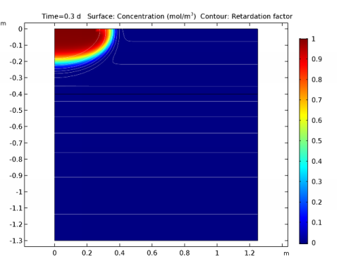
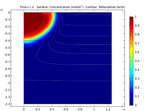
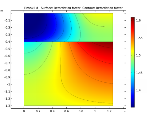
In the Settings window for Contour, click Replace Expression in the upper-right corner of the Expression section. From the menu, choose Model>Component 1>Transport of Diluted Species in Porous Media>tds.RF_c - Retardation factor.
|
|
3
|
|
4
|
|
5
|
|
6
|
|
7
|
|
8
|
|
9
|
|
10
|
|
1
|
|
2
|
|
3
|
|
4
|
|
1
|
|
2
|
|
3
|
|
1
|
|
2
|
In the Settings window for Surface, click Replace Expression in the upper-right corner of the Expression section. From the menu, choose Model>Component 1>Transport of Diluted Species in Porous Media>tds.RF_c - Retardation factor.
|
|
3
|
|
4
|
|
1
|
|
2
|
|
3
|
|
4
|