
|
|
|
|
1
|
|
2
|
|
3
|
Click Add.
|
|
4
|
Click Study.
|
|
5
|
|
6
|
Click Done.
|
|
1
|
|
2
|
|
3
|
|
4
|
Browse to the model’s Application Libraries folder and double-click the file compression_ignition_parameters.txt.
|
|
1
|
In the Model Builder window, under Component 1 (comp1) right-click Definitions and choose Variables.
|
|
2
|
|
3
|
|
4
|
Browse to the model’s Application Libraries folder and double-click the file compression_ignition_variables.txt.
|
|
1
|
|
2
|
|
3
|
|
4
|
|
5
|
Click to expand the Discretization section. Select the Uniform scaling of concentration variables check box.
|
|
6
|
|
1
|
|
2
|
In the Settings window for Reversible Reaction Group, click to expand the CHEMKIN import for kinetics section.
|
|
3
|
|
4
|
Click Browse.
|
|
6
|
Click Import.
|
|
1
|
In the Model Builder window, expand the Component 1 (comp1)>Reaction Engineering (re)>Species Group 1 node, then click Species Thermodynamics 1.
|
|
2
|
In the Settings window for Species Thermodynamics, click to expand the CHEMKIN import for thermodynamic data section.
|
|
3
|
|
5
|
Click Import.
|
|
1
|
In the Model Builder window, under Component 1 (comp1)>Reaction Engineering (re) click Initial Values 1.
|
|
2
|
|
3
|
|
4
|
|
1
|
|
2
|
|
3
|
|
4
|
|
5
|
|
1
|
|
2
|
|
3
|
|
4
|
|
5
|
|
6
|
|
7
|
|
1
|
|
2
|
In the Settings window for Global, click Replace Expression in the upper-right corner of the y-axis data section. From the menu, choose Model>Component 1>Reaction Engineering>comp1.re.c_N2 - Concentration.
|
|
3
|
Click Add Expression in the upper-right corner of the y-axis data section. From the menu, choose Model>Component 1>Reaction Engineering>comp1.re.c_CH4 - Concentration.
|
|
4
|
Click Add Expression in the upper-right corner of the y-axis data section. From the menu, choose Model>Component 1>Reaction Engineering>comp1.re.c_O2 - Concentration.
|
|
5
|
Click Add Expression in the upper-right corner of the y-axis data section. From the menu, choose Model>Component 1>Reaction Engineering>comp1.re.c_CH2O - Concentration.
|
|
6
|
Click to expand the Coloring and style section. Locate the Coloring and Style section. In the Width text field, type 2.
|
|
7
|
|
9
|
|
10
|
|
1
|
|
2
|
|
3
|
|
1
|
|
2
|
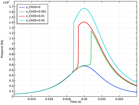
In the Settings window for Global, click Replace Expression in the upper-right corner of the y-axis data section. From the menu, choose Model>Component 1>Reaction Engineering>comp1.re.p - Pressure.
|
|
3
|
|
1
|
|
2
|
|
3
|
|
4
|
|
5
|
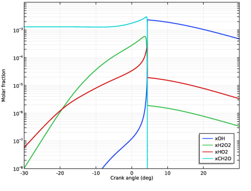
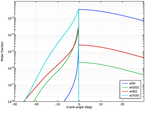
In the associated text field, type Crank angle (deg).
|
|
6
|
|
7
|
In the associated text field, type Molar fraction.
|
|
1
|
|
2
|
In the Settings window for Global, click Replace Expression in the upper-right corner of the y-axis data section. From the menu, choose Model>Component 1>Reaction Engineering>comp1.re.c_OH - Concentration.
|
|
3
|
|
4
|
|
5
|
|
6
|
Click to expand the Coloring and style section. Locate the Coloring and Style section. In the Width text field, type 2.
|
|
7
|
|
1
|
|
2
|
|
3
|
|
4
|
|
1
|
|
2
|
|
1
|
|
2
|
|
1
|
|
2
|
|
5
|
|
1
|
|
2
|
|
3
|
|
4
|
|
5
|
|
6
|
|
7
|
|
8
|
|
9
|
|
1
|
|
2
|
|
1
|
|
2
|
|
1
|
|
2
|
|
3
|
Click Add.
|
|
5
|
|
6
|
|
7
|
|
8
|
|
1
|
|
2
|
|
3
|
|
4
|
|
5
|
Click to expand the Legend section. Locate the Axis section. Select the Manual axis limits check box.
|
|
6
|
|
7
|
|
8
|
|
9
|
|
10
|
|
1
|
|
2
|
|
3
|
|
4
|
|
6
|
|
1
|
|
2
|
|
1
|
|
2
|
|
4
|
|
1
|
|
2
|
|
3
|
|
1
|
|
2
|
|
4
|
|
1
|
|
2
|
|
1
|
|
2
|
|
4
|
|
1
|
|
2
|
|
3
|
|
1
|
|
2
|
|
4
|