|
|
|
|
1
|
|
2
|
|
3
|
Click Add.
|
|
4
|
Click Study.
|
|
5
|
|
6
|
Click Done.
|
|
1
|
|
2
|
|
1
|
|
2
|
|
3
|
Click Browse.
|
|
4
|
Browse to the model’s Application Libraries folder and double-click the file generator_2d.mphbin.
|
|
5
|
Click Import.
|
|
1
|
|
2
|
|
3
|
|
4
|
|
1
|
|
1
|
|
2
|
|
3
|
In the tree, select Built-In>Air.
|
|
4
|
|
1
|
|
2
|
|
3
|
|
1
|
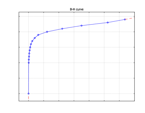
In the Model Builder window, under Component 1 (comp1)>Materials click Soft Iron (without losses) (mat2).
|
|
3
|
|
1
|
|
2
|
|
3
|
|
1
|
Right-click Component 1 (comp1)>Rotating Machinery, Magnetic (rmm) and choose Prescribed Rotational Velocity.
|
|
3
|
In the Settings window for Prescribed Rotational Velocity, locate the Prescribed Rotational Velocity section.
|
|
4
|
|
1
|
In the Model Builder window, right-click Rotating Machinery, Magnetic (rmm) and choose the domain setting Vector Potential>Ampère’s Law.
|
|
3
|
|
4
|
|
5
|
Locate the Magnetic Field section. From the Constitutive relation list, choose Remanent flux density.
|
|
6
|
|
7
|
Right-click Component 1 (comp1)>Rotating Machinery, Magnetic (rmm)>Ampère’s Law 2 and choose Rename.
|
|
8
|
|
9
|
Click OK.
|
|
1
|
In the Model Builder window, right-click Rotating Machinery, Magnetic (rmm) and choose the domain setting Vector Potential>Ampère’s Law.
|
|
3
|
|
4
|
|
5
|
Locate the Magnetic Field section. From the Constitutive relation list, choose Remanent flux density.
|
|
6
|
|
7
|
Right-click Component 1 (comp1)>Rotating Machinery, Magnetic (rmm)>Ampère’s Law 3 and choose Rename.
|
|
8
|
|
9
|
Click OK.
|
|
1
|
In the Model Builder window, right-click Rotating Machinery, Magnetic (rmm) and choose the domain setting Vector Potential>Ampère’s Law.
|
|
2
|
|
3
|
|
5
|
Right-click Component 1 (comp1)>Rotating Machinery, Magnetic (rmm)>Ampère’s Law 4 and choose Rename.
|
|
6
|
|
7
|
Click OK.
|
|
1
|
In the Model Builder window, right-click Rotating Machinery, Magnetic (rmm) and choose the domain setting Vector Potential>Coil.
|
|
3
|
|
4
|
|
5
|
|
6
|
|
7
|
|
8
|
|
1
|
Right-click Component 1 (comp1)>Rotating Machinery, Magnetic (rmm)>Coil 1 and choose Reversed Current Direction.
|
|
2
|
|
1
|
In the Model Builder window, right-click Rotating Machinery, Magnetic (rmm) and choose Pairs>Continuity.
|
|
2
|
|
3
|
|
1
|
In the Model Builder window, under Component 1 (comp1) right-click Mesh 1 and choose Free Triangular.
|
|
2
|
|
3
|
|
4
|
Click the Custom button.
|
|
5
|
|
6
|
|
1
|
|
2
|
|
3
|
|
1
|
|
2
|
|
3
|
|
4
|
|
5
|
Find the Algebraic variable settings subsection. From the Error estimation list, choose Exclude algebraic.
|
|
6
|
In the Model Builder window, expand the Study 1>Solver Configurations>Solution 1 (sol1)>Time-Dependent Solver 1 node, then click Fully Coupled 1.
|
|
7
|
|
8
|
Click to expand the Method and termination section. Locate the Method and Termination section. From the Jacobian update list, choose Once per time step.
|
|
9
|
|
10
|
|
1
|
|
2
|
|
3
|
|
1
|
|
2
|
|
3
|
|
4
|
|
1
|
|
2
|
|
3
|
|
4
|
|
5
|
|
6
|
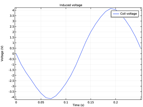
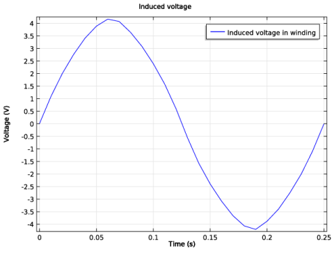
In the associated text field, type Time (s).
|
|
7
|
|
8
|
In the associated text field, type Voltage (V).
|
|
1
|
|
2
|
In the Settings window for Global, click Replace Expression in the upper-right corner of the y-axis data section. From the menu, choose Component 1>Rotating Machinery, Magnetic (Magnetic Fields)>Coil parameters>rmm.VCoil_1 - Coil voltage.
|
|
3
|