The Multibody Dynamics Interface
The Multibody Dynamics (mbd) interface (), found under the Structural Mechanics branch () when adding a physics interface, is intended for analysis of mechanical assemblies. The parts in the assembly can be rigid or flexible, and are connected by various types of joints, gears, springs, or dampers. Flexible parts can be defined using solid, shell or beam elements. There are many types of joints, such as hinges or ball joints, which can be used based on the type of connection required between components. There are many types of gears, such as spur, helical, bevel, worm, or rack, which can be used for power transmission. Computed results are displacements, velocities, accelerations, joint forces, gear contact forces and — in flexible parts — stresses. The joints can be given properties such as spring constants, damping, friction, and limits on movement. The gears pairs can also be given properties such as gear mesh stiffness, mesh damping, backlash, transmission error, and friction.
The Linear Elastic Material is the default material model. It adds the equations for the displacements in a linear elastic solid and has a Settings window to define the elastic and inertia properties of a material. As an alternative, a domain can be made into a rigid body, using the Rigid Domain material mod — el. A rigid domain adds the rigid body dynamics equations and has a Settings window to define inertia properties of a material.
With the Nonlinear Structural Materials Module, you can also incorporate nonlinear material models like hyperelasticity or plasticity by adding a Solid Mechanics interface to the model.
When the Multibody Dynamics interface is added, these default nodes are also added to the Model BuilderLinear Elastic Material, Free (a boundary condition where boundaries are free, with no loads or constraints), and Initial Values (only applicable for flexible domains). Then, from the Physics toolbar, add features that implement other multibody dynamics properties. You can also right-click Multibody Dynamics to select physics features from the context menu.
Settings
The Label is the default physics interface name.
The Name is used primarily as a scope prefix for variables defined by the physics interface. Refer to such physics interface variables in expressions using the pattern <name>.<variable_name>. In order to distinguish between variables belonging to different physics interfaces, the name string must be unique. Only letters, numbers and underscores (_) are permitted in the Name field. The first character must be a letter.
The default Name (for the first physics interface in the model) is mbd.
2D Approximation
From the 2D approximation list select Plane stress or Plane strain (the default). Plane stress is relevant for structures which are thin in the out-of-plane direction, such as a thin plate. Plane strain is relevant when the 2D model can be considered as a cut through an object which is long in the out-of-plane direction. This information is needed if the components are flexible and modeled using Linear Elastic Material. For more information see the theory section.
Thickness
For 2D components, enter a value or expression for the Thickness d. The default value of 1 m is suitable for plane strain models, where it represents a unit-depth slice, for example. For plane stress models, enter the actual thickness, which should be small compared to the size of the plate for the plane stress assumption to be valid. In Acoustic-Structure Interaction problems, the Thickness should be set to 1 m.
Use a Change Thickness node to change thickness in parts of the geometry if necessary.
Structural Transient Behavior
From the Structural transient behavior list, select Include inertial terms or Quasi-static. Use Quasi-static to treat the mechanical behavior as quasi-static (with no mass effects — that is, no second-order time derivatives). Selecting this option gives a more efficient solution for problems where the variation in time is slow when compared to the natural frequencies of the system.
Reference Point for Moment Computation
Enter the coordinates for the Reference point for moment computation xref (variable refpnt). The resulting moments (applied or as reactions) are then computed relative to this reference point. During the results and analysis stage, the coordinates can be changed in the Parameters section in the result nodes.
Initial Values
Specify initial values for a rigid body translation and rotation. The values specified here are, as a default, inherited by the initial values settings for Rigid Domain and Linear Elastic Material.
For 3D components only: Axis of rotation Ω.
Angular velocity ω (3D components) and φ/t (2D components)
Joints Summary
This is an information table that displays the name of all the joints used in a model and their source and destination attachments. This table summarizes all the connections present in a model and can be used to review the connections.
Rigid Body DOF Summary
This is an information table that displays the number of degrees of freedom and constraints introduced by rigid domains and joints. You can use this information to determine whether you model has an appropriate number of constraints or not when running pure rigid body analysis.
The contents of the columns are:
N: The number of features of a certain type.
DOF: The number of degrees of freedom added to the model by all features of this type.
Prescribed: The number of degrees of freedom controlled by Prescribed Motion and similar conditions for all features of this type.
Constraints: The number of constraints for all features of this type. Both internal constraints and constraints added explicitly by for example Fixed conditions are included.
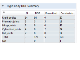
The last two rows of the table contain a summary. In the Total row, the number of DOFs, prescribed conditions and constraints are summed.
The Net row contains the net number of degrees of freedom of the model, that is the difference between all degrees of freedom and the constraints and prescribed motions. A negative net number of degrees of freedom indicates that the mechanism is over-constrained and is not shown. In that case, the net number of constraints is instead displayed.
Some constraints are conditional and are not present during the whole analysis. Such constraints are counted in the summary table, irrespective of their actual status.
The contents of the table do not change if you suppress any of the contributing features from the settings in the study step.
In general, and if there are flexible bodies in the system, the model’s total number of degrees of freedom increase significantly. Such degrees of freedom are not accounted for in the summary.
Dependent Variables
The physics interface uses the global spatial components of the Displacement field u as dependent variables in the flexible domains. The default names for the components are (u, v, w) in 3D. In 2D the component names are (u, v), and in 2D axial symmetry they are (u, w). You can however not use the “missing” component name in the 2D cases as a parameter or variable name because it is still used internally.
You can change both the field name and the individual component names. If a new field name coincides with the name of another displacement field, the two fields (and the interfaces which define them) share degrees of freedom and dependent variable component names. You can use this behavior to connect a Multibody Dynamics interface to a Shell directly attached to the boundaries of the solid domain, or to a Solid Mechanics interface sharing a common boundary.
A new field name must not coincide with the name of a field of another type (that is, it must contain a displacement field), or with a component name belonging to some other field. Component names must be unique within a model except when two interfaces share a common field name.
Each rigid domain, attachment, and joint also adds a number of global dependent variables depending on the number of ODEs needed to represent its motion.
Discretization
To display this section, click the Show button () and select Discretization.
In the Multibody Dynamics interface you can choose not only the order of the discretization, but also the type of shape functions: Lagrange or serendipity. For highly distorted elements, Lagrange shape functions provide better accuracy than serendipity shape functions of the same order. The serendipity shape functions will however give significant reductions of the model size for a given mesh containing hexahedral, prism, or quadrilateral elements.
The discretization order applies to the flexible bodies. The default is to use Linear shape functions for the Displacement field. If you want to compute stresses with good accuracy, increase the shape function order to Quadratic serendipity or Quadratic.