COMSOL 6.4 - Results

First, look at the modes polarized in the z direction.

1

In the Model Builder window, expand Electric Mode Field, Port 1 (ewbe)

, and then select Surface 1

2

In the Settings window for Surface, click Replace Expression

in the upper-right corner of the Expression section. From the menu, navigate to and select the variable Model > Component 1 > Electromagnetic Waves, Beam Envelopes, Unidirectional > Boundary mode analysis > Boundary mode electric field - V/m > ewbe.tEbm1z - Boundary mode electric field, z-component.

3

Locate the Coloring and Style section. From the Color Table list, choose Wave > WaveLight.

4

In the Model Builder, click Electric Mode Field, Port 1 (ewbe)

5

In the Settings window for 3D Plot Group locate the Data section. From the Effective mode index list, choose the largest effective index. This is the last value in the list. Since the modes are pairwise (almost) degenerate, the value to pick is 3.4717.

6

Click the Plot button

. The plot below shows the symmetric mode polarized in the z direction (same as Figure 15 in Results and Discussion).

Notice that your plot may look different from the plot above, as the plot shows the real part of the boundary mode electric field. The computed complex electric field can have a different phase factor than for the plot above. Thus, the field can either show minima (a blue color) or maxima (a red color) at the locations for the waveguide cores. However, since this is a symmetric mode, it will have the same field values for both waveguide cores.

Another consequence of the arbitrary phase factor is that the magnitude for the displayed real part of the electric field in your plot can be different from what is shown in the plot above.

When adding two mode fields having arbitrary phases, the resulting superposition field will, of course, also have a random shape. To remove this arbitrariness, later, in the last part of this example model, the Port input power and the Mode phase parameters for the exciting ports will be used to ensure that the superposition field approximates a target field.

7

From the Effective mode index list, choose the third largest effective index. This is the second value in the list (3.4714).

8

button. The plot below shows the anti-symmetric mode polarized in the z direction (same as Figure 16 in Results and Discussion).

9

In the Model Builder, under Electric Mode Field, Port 1 (ewbe)

, click Surface 1

10

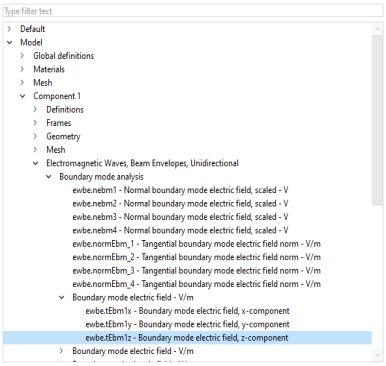
From the Settings window for Surface, locate the Expression section and enter ewbe.tEbm1y in the Expression text field, to plot the mode field polarized in the y direction.

11

In the Model Builder click Electric Mode Field, Port 1 (ewbe)

12

In the Settings window for 3D Plot Group, locate the Data section. From the Effective mode index list, choose the second largest effective index. This is the third value in the list (3.4717).

13

Click the Plot button

. The plot below shows the symmetric mode polarized in the y direction (same as Figure 17 in Results and Discussion).

14

From the Effective mode index list, choose the smallest effective index (the first value in the list, 3.4714)

15

Click the Plot button

. The plot below shows the anti-symmetric mode polarized in the y direction (same as Figure 18 in Results and Discussion).

You will need to copy the effective indices for the different modes and use them in the boundary mode analyses for the different ports.

1

In the Results toolbar, select Global Evaluation

2

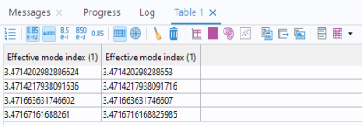
Locate the Expressions section in the Settings window for Global Evaluation and enter ewbe.neff_1 in the Expression cell for the first table row. The variable ewbe.neff_1 is the effective index for the first port.

3

Click the Evaluate button

Now, copy all information in the table to the clipboard. Then paste that information into your favorite text editor, so you can easily enter the values later in the boundary mode analysis steps.

4

In the Table window, click Full Precision

5

In the Table window, click Copy Table and Headers to Clipboard

6

Paste the contents of the clipboard into your text editor for later reference.