The Thin Layer node is used to identify boundaries that have a thin layer attached to them. These boundaries may either be exterior or interior boundaries to the domain where the physics interface is active. The
Thin Layer node also determines the thickness of the thin layer, and how to approximate the deformation gradient on it. The first choice is whether to use a
Layered or a
Nonlayered thin structure.
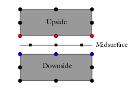
In the majority of cases, the Nonlayered approximation is sufficient to capture the behavior of the thin layer. For this type of layer, two sets of degrees of freedom (DOFs) are introduced at the boundary; one set corresponds to the upside, and one set to the downside as illustrated in
Figure 2-41. In COMSOL Multiphysics, this is referred as a slit of the displacement field on the thin layer boundary.
Note that in Figure 2-41 no extra integration points are introduced in the through-thickness direction, and that numerical integration is made on the midsurface. Hence, dependent variables always have a linear variation in the thickness direction; that is, their gradients are constant in the through-thickness direction. This also applies to inelastic quantities such as plastic strains.
The Layered type can be used when a more detailed description of the through-thickness behavior is needed. For this type of thin layer, a slit of the displacement field is made on the boundary, and additional DOFs are introduced between the upside and downside as illustrated in
Figure 2-42. These extra DOFs facilitate a more detailed through-thickness representation of stresses and strains, and they make it possible to, for example, model composites and laminate strata. Continuity is enforced by constraints between the DOFs on the upside and the downside, and the extra DOFs. The through-thickness discretization is controlled by the attached material. For more details about modeling layered structures, see
Composite Materials Modeling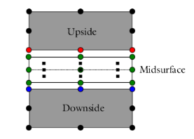
When the Nonlayered type is used, it is possible to choose different approximations of the deformation measure in the thin layer:
The description in Figure 2-41 is representative of the solid and spring approximations. The solid approximation is the most general and accounts for the full normal and tangential deformations in the thin layer. The spring approximation is similar but neglects the membrane deformation. This is useful for cases where the behavior of the thin layer is given by force versus extension data, as is often the case when modeling gaskets.