COMSOL 6.4 - Working with CMS Models

A reduced component can be created in an applicable physics interface by adding a node, in which you select all domains that are to be reduced, as shown in Figure 2-30. Subsequently, one subnode should be added for each set of domains for which a reduced-order model (ROM) is to be generated. By default, this step is automated and the selected domains are grouped into disconnected components as detected from the geometry. With this setting, a number of subnodes are created and their selections are set automatically. However, by setting to in the node, you can take manual control of the geometric definition of the components by adding, removing, or modifying nodes. In each such node, select a number of domains that defines a component. This may be necessary if domains are not physically adjacent, but connected by other means, for example, by springs.

By default, disconnected geometries connect by the and pair features are merged when automatically generating subnodes. This also applies to , , and connection features in the Shell interface. The automatic handling of such connections can be disabled by clearing in the node.

Figure 2-30: A Reduced Flexible Components node with two automatically generated Component Definition subnodes.

•

If the components are geometrically disjoint, then should be used in the geometry sequence. If not, is probably a better choice, but then you may have to either create unions between domains that are part of the same components, or edit the settings in the nodes manually.

•

In the majority of cases, it is sufficient with one node per physics interface. If you, however, do not want to train all ROMs in one sweep, having a single node per actual component can be useful. Another case is if you decide to reduce one additional component after already having reduced one or several other components. Then, adding an additional node can be an alternative.


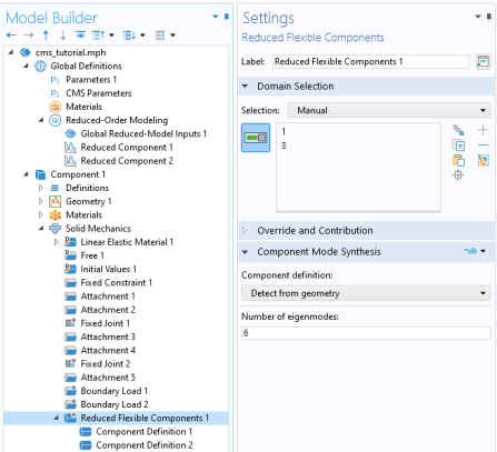
	The Reduced Flexible Components node is only applicable on domains where the material behavior is determined by a Linear Elastic Material node or a Section Stiffness node in the Shell interface. You can, however, have several such nodes with different properties and settings within one reduced component.

A disconnected reduced component, as defined by a subnode, can only be connected to other parts of the geometry by attachment features. In fact, to be able to create the ROM, each component must be connected to at least one node. By using attachments, a reduced component can be connected to any number of other parts, reduced or full, of the model assembly.


	See also Attachments.

When working with CMS, the full static and dynamic behavior of a component is represented by a number constraint modes and constrained eigenmodes that are computed in the training phase. These are independent of each other and are used to construct one ROM for each component. Each node connected to a component will add a number of static load cases that describe the constraint modes: six in 3D, and three in 2D. The number of eigenmodes to be used is controlled manually. You can either define it for all components in the node, or individually in each subnode. To get an accurate representation of the reduced component, always make sure to use a sufficient number of eigenmodes to describe the dynamics of each component. During the eigenfrequency training step, all attachments are treated as fixed constraints, hence, the eigenmodes are always constrained.

Note that, from a computational point of view, each eigenmode is represented as a degree of freedom when using the reduced component in a global analysis. For computational efficiency, you should avoid using unnecessarily many eigenmodes.

To create the ROMs, a special study sequence needs to be set up for each node. It should sweep over all subnodes, and for each component, compute the static load cases and the requested eigenmodes in training study steps as outlined above. The results from these study steps are then used in a step to generate a ROM. By using the (

) button in the node, the setup of this special study sequence is automated. In the model tree, a generated ROM is represented as a node with the label under as seen in Figure 2-31.

Figure 2-31: Nodes in the model tree that are added automatically when working with CMS.

•

When a node is added, a set of parameters are also automatically added under the branch. These are placed in the node seen in Figure 2-31, which is created by the first node in the model. Additionally, each node creates an explicit selection node with the label in its model component. The parameters and selection are used in the corresponding CMS study and should therefore not be deleted or modified. As a safeguard, they are regenerated if missing when the (

) action is executed.

•

If you change the number of nodes or add new features to the physics interface after setting up the CMS study and want to run it again, the safest option is to reconfigure the study by using the (

) action. Note that this will delete any ROMs that have previously been generated. To save these in the model, you can temporarily change the name of the existing nodes under before reconfiguring the CMS study.

Applying Loads to Reduced Components

Loads can be applied to a reduced component in two fundamentally different ways:

External to the ROM: In this case, the weak contribution of the load on the reduced component is part of the assembly procedure for the global FE model. This is the default choice and can handle any type of loads. It is, however, the computationally more expensive of the two methods.

Internal to the ROM: The load can either be constant or a function of a global reduced model input. In this case, the load is stored as part of the ROM.

Be careful not to mix up the two alternatives; doing so can lead to double load contributions. For this reason, option 1 is usually recommended. When the (

) button is used, all load type features are disabled in the study steps of the CMS study.

Figure 2-32: Loads are, by default, disabled in the model reduction study.

The advantage of option 2 is that it can be computationally cheaper in the global analysis, since any evaluation of weak equations in domains of the reduced component is avoided. To use this approach, enable the relevant load features in the reference study step to the study step in the CMS study. The same load features should then be disabled in all other studies. By selecting in the node, you can change the default behavior of loads when the (

) button is used. When selected, all loads are enabled in the study steps of the generated CMS study.

You can find an example of both approaches for load application in this tutorial model:

•

Component Mode Synthesis Tutorial: Application Library path

•

Component Mode Synthesis Tutorial: Application Library path

•

Component Mode Synthesis Tutorial: Application Library path

While conceptually similar to other load features, , , and are always considered as internal to the ROM and part of the reduced component. They are, by default, enabled in the when using the (

) button. The reason is that they are considered to contribute to the acceleration of the frame. If necessary, use control inputs to parameterize, for example, the gravity vector or rotation speed.

The CMS Study

The CMS study is a parametric sweep over a set of components as defined by the subnodes of a node with the aim to create one ROM for each component. The study is automatically generated by using the (

) button in a node. The auto-generated study and solver sequences have a number of built-in features and settings that greatly simplifies the process of creating a reduced component; especially when there are multiple components to be reduced. The study sequence is shown in Figure 2-33 and consists of:

•

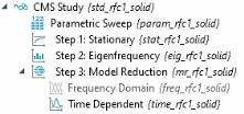
A over the components to be reduced

•

A training study step to compute the constraint modes from the static load cases

•

An training study step to compute the constrained eigenmodes

•

A study step to generate the ROM. This step can either use a or study step as a reference.

Figure 2-33: The automatically generated CMS study.


	If the global model is to be used in a frequency domain analysis, use a Frequency Domain study step as a reference during model reduction. If not, use a Time Dependent study step. Both steps are added by the Configure CMS study () action, and can be enabled or disabled depending on the use case. By default, the Time Dependent study step is enabled.

Key to the CMS study is that all study steps are solved on a subset of the total model; the selection of the component. This is controlled in the nodes of the solver sequence. When using an auto-generated CMS study, the selections used are automatically updated during the sweep over components.

Running a CMS study creates a number of datasets in the branch as well as subnodes to the node under .

•

The datasets contains the solution that is used to create a ROM, including the constraint modes and eigenmodes. It also contains the matrices of the ROM, which can be inspected by using the derived values node.

•

Depending on the chosen reference study step during model reduction, or nodes are created under . When created from a CMS Study, these are always created with a default label and names that are related to the generating study and physics. Moreover, the CMS study generates ROMs with a stateful interface, which is a requirement for it to connect to other parts of the model. You can use and other settings in the generated ROMs to modify their behavior when used in a global analysis.


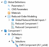
	Once the ROMs have been created, you can in principle delete the CMS study to clean up the model tree. In fact, you only need to keep the Reduced Flexible Components node and the generated ROMs under Global Definitions.


	Neither the names, nor the order of the list of ROMs in the Reduced-Order Modeling node under Global Definitions should be changed, as this will break the connection between the ROMs, the physics, and the reduced component. The automatic naming convention has the structure <rom>_n_<feat>_<phys>_<i>, where <rom> is a generic tag for the generating ROM, <feat> is the tag of the Reduced Flexible Components node that generated the CMS study, <phys> is the physics tag, and <i> is a number. For example, the ROM of the first component in a Solid Mechanics interface is typically named rom1_n_rfc1_solid_1.

Setting up the Global Model

Using ROMs created from a node and a CMS Study in a global model, in general, requires no further steps to be taken. The only requirement is that the states of the ROMs are solved together with the other dependent variables of the model. By default, the status of these ROMs are synchronized with the status of the generating physics in non-CMS studies, which takes care of this requirement.


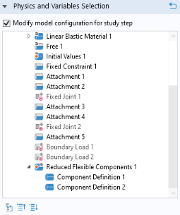
	If all the domains of the physics interface are reduced, it is possible to turn off the synchronization of the Solve for status, since in such cases it is only necessary to solve for the states of the ROMs. By not solving for the dependent variables of the physics, it is made sure that no double contributions are added by, for example, load features. Clear the Synchronize ‘Solve for’ study setting for Reduced Components checkbox in the Reduced Flexible Components node to make this possible.

One way to add more control over the behavior of a ROM is to add control inputs in under . These should be added to the model before solving the CMS study, and can be used in expressions in relevant physics nodes. After running the CMS study, you can modify the input expression for each added control input, either globally or individually in each of the generated nodes.


	If you include a load in a reduced component, and enter a value or a parameter for its amplitude, then that load will have a constant value when the component is reused. If you want to be able to, for example, make that load time dependent, or to switch it off, then you define it using a control input.


	For a more detailed discussion on how to work with ROM control inputs and their limitations, see Reduced-Order Model Inputs in the COMSOL Multiphysics Reference Manual.

Important Considerations

A number of important considerations to be aware of when working with CMS and reduced components are listed below:

•

Do not modify the content of automatically generated nodes in the model tree, such as the node, and the selection.

•

Only zero-valued constraints can be applied to a reduced component. While it is fundamentally possible to apply constraints on a reduced component in a global analysis, the correct way is to apply them when generating the ROMs in a CMS study so that such constraints can be accounted for while computing constraint modes and eigenmodes. Later, constraints can be removed in all other studies. This is handled automatically for most such features including for example:

No constraint equations are added for these features on selections that intersect that of a node. For the node and similar features, any nonzero values set for the constraint are, moreover, ignored in the CMS study.

•

nodes can be used without a connection to other parts of the model to define additional static modes of the reduced component. Note that attachments by default induce a rigid boundary on its selection.

•

, , and are special features that add either mass or stiffness to the reduced component, and can therefore be considered as part of its basic properties. By default, these are enabled in the when using the (

) button. No mass nor stiffness is added in a global study on selections intersecting with that of a node.

•

When working with CMS, the following subnodes to and are supported when creating reduced components:

All other subnodes are, by default, disabled in the when using the (

) button. Some options in the supported features may, however, not be supported. For example, the option in is not supported with CMS.

•

In the subnode to or , the following are supported:

When using the (

) button, the subnode is disabled in the training steps to avoid complex eigenpairs, but active in the reference step to the model reduction. Any contributions are removed on selections that intersects with that of a node in a global study.

•

Damping can also be added to reduced components by , , and nodes. For these features, damping contributions are only added on selections intersecting with that of a node in the reference step to the model reduction. No contributions are added in the training steps for such selections to avoid complex eigenpairs.

•

Reduced components are by definition linear. Do not use any features that are nonlinear such as , , or on the same selection as a node. Also, make sure not to induce nonlinearity by user defined expressions in features that are to be reduced. This also applies to boundary, edge, and point features adjacent to the domains selected in a node.

•

It is not possible to compute dissipated energy due to for example damping on selections that intersect that of a node. The setting is ignored for such selections.

•

Certain features that add weak contributions on domain, boundary, edge, or point level should be used with care if their selections intersect that of a node. To get consistent results and avoid double contributions, it may be necessary to manually disable some features in the model tree of the training study step of a generated CMS study, or in the global study that uses a ROM. Examples of such features, other than loads, include . By default, these are disabled in the when using the (

) button.

•

Most features that add global dependent variables are not applicable together with reduced components. The reason is that it is difficult to automatically determine to which part of the model such variables belong. Hence, do not use features such as , , , , or when setting up reduced components. By default, all such features are disabled in the when using the (

) button. The only exception is the feature which is specially designed to work with reduced components.

•

Features and functionality that add dependent variables which are expected to have a significantly different order of magnitude compared to the displacements should be used with caution when creating reduced components. The reason is that such DOFs can corrupt the scaling of the eigenvectors used to train the ROM during model reduction, which in the end will result in an inaccurate ROM. Examples of functionality that may cause this are:

The mixed formulation in

The connection type in nodes

The Lagrange multipliers added by weak constraints

If such functionality must be used, you can try to manually adjust the scaling of the eigenvectors by changing the in the of the . Another alternative is the try setting to .

•

Translating or rotating a ROM is not supported. Hence you cannot use a single ROM to represent multiple reduced components.

•

Import of ROMs created in another COMSOL Multiphysics model or any external software is not supported for reduced components.