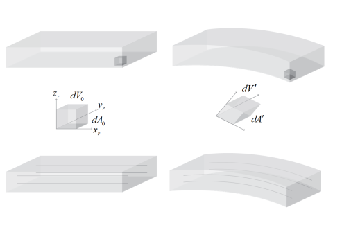
COMSOL 6.4 - Geometric Nonlinearity, Frames, and the ALE Method

Consider the bending of a beam in the general case of a large deformation (see Figure 2-24). In this case the deformation of the beam introduces an effect known as geometric nonlinearity into the equations of solid mechanics.

Figure 2-24 shows that as the beam deforms, the shape, orientation, and position of the element at its tip changes significantly. Each edge of the infinitesimal cube undergoes both a change in length and a rotation that depends on position. Additionally, the three edges of the cube are no longer orthogonal in the deformed configuration (although typically for practical strains the effect of the nonorthogonality can be neglected in comparison to the rotation).

From a simulation perspective it is possible to solve the equations of solid mechanics on either a fixed domain (this is often called a Total Lagrangian formulation), or on a domain that changes continuously with the deformation. The latter approach is often called an Updated Lagrangian formulation. These two approaches also stand in contrast to the Eulerian formulation, which is often used for fluid mechanics. In an Eulerian formulation, the flow through a domain fixed in space is considered, while in the Lagrangian formulation, a fixed volume of material is considered.

	In COMSOL Multiphysics, the concepts of a material frame and a spatial frame are used. Equations formulated in the material frame will give a Total Lagrangian formulation, while equations formulated in the spatial frame will give an Eulerian formulation. See Frames and Coordinate Systems in the Structural Mechanics Theory chapter for more details.

Solid mechanics in COMSOL Multiphysics is formulated on the material frame. This is achieved by defining a displacement field for every point in the solid, usually with the components u, v, and w. At a given coordinate (X, Y, Z) in the reference configuration (on the left of Figure 2-24), the value of u describes the displacement of the point relative to its original position. The displacement is considered as a function of the material coordinates (X, Y, Z), but it is not explicitly a function of the spatial coordinates (x, y, z). The spatial coordinates give the current location in space of a point in the deformed solid. As a consequence, it is only possible to compute derivatives with respect to the material coordinates.

Taking derivatives of the displacement with respect to X, Y, and Z enables the definition of a strain tensor. There are possible representations of the deformation. Any reasonable representation must however be able to represent a rigid rotation of an unstrained body without producing any strain. The engineering strain fails here, thus it cannot be used for general geometrically nonlinear cases. One common choice for representing large strains is the Green–Lagrange strain. It contains derivatives of the displacements with respect to the original configuration. The values therefore represent strains in material directions. This choice allows a physical interpretation, but it must be realized that even for a uniaxial case, the Green–Lagrange strain is strongly nonlinear with respect to the displacement. If an object is stretched to twice its original length, the Green–Lagrange strain is 1.5 in the stretching direction. If the object is compressed to half its length, the strain would read −0.375.

An even more fundamental quantity is the deformation gradient, which contains the derivatives of the deformed coordinates with respect to the original coordinates:

The deformation gradient contains all information about the local deformation in the solid, and can be used to form many other strain quantities. As an example, the Green–Lagrange strain is

An element at a point (X, Y, Z) specified in the material frame moves with a single piece of material throughout a solid mechanics simulation. It is often convenient to define material properties in the material frame as these properties move and rotate naturally together with the volume element at the point at which they are defined as the simulation progresses. In Figure 2-24 this point is illustrated by the small cube highlighted at the end of the beam, which is stretched, translated, and rotated as the beam deforms. The three mutually perpendicular faces of the cube in the Lagrange frame are no longer perpendicular in the deformed (spatial) frame. The deformed frame coordinates in this frame are denoted (x, y, z) in COMSOL.

	It is important to note that, as the solid deforms, the Lagrangian frame becomes a nonorthogonal curvilinear coordinate system (see the lower part of Figure 2-24 to see the deformation of the X-axis). Particular care is therefore required when defining physics in this coordinate system.

Under geometric nonlinearity, a Solid Mechanics interface (or a similar structural mechanics interface such as Multibody Dynamics) will assume control over the spatial frame in the domains where it is active. However, the definition of the spatial frame must be unique, and there may be conflicts. Some examples are:

•

A Solid Mechanics interface and a moving mesh feature (for example, or ) have a common selection. In this case, the selection in the Solid Mechanics interface will be marked as “not applicable”. Thus, it is not possible to solve a structural mechanics problem on such a domain.

When two physics interfaces are competing for frame control, you will get the error message “Multiple moving frame specifications on the same selection” when trying to run the study. To identify the problem, go to the settings for the study step, and select . There, you will get an overview of the frame control in the model. Note that it is quite possible that several features control the spatial frame, as long as it is on different geometric selections.

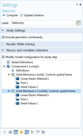
When you select a physics interface in the tree view, you can click the button (

) to toggle whether that interface should control the spatial frame or not.

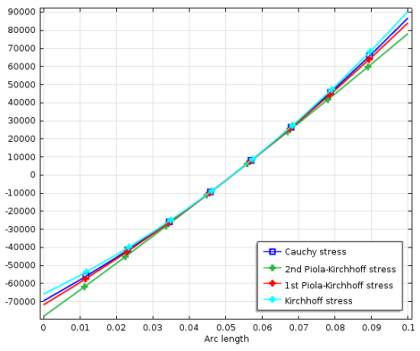
For example, in the spatial frame it is easy to define forces per reference area (known as tractions) that act within the solid and to define a stress tensor that represents all of these forces that act on a volume element. Such forces could be physically measured, for example, using an implanted piezoresistor. The stress tensor in the spatial frame is called the Cauchy or true stress tensor (in COMSOL Multiphysics this is referred to as the spatial stress tensor). To construct the stress tensor in the Lagrangian frame a tensor transformation must be performed on the Cauchy stress. This produces the second Piola–Kirchhoff (or material) stress, which can be used with the material strain to solve the solid mechanics problem in the (fixed) material frame. This is how the Solid Mechanics interface works when geometric nonlinearities are enabled.

For the Cauchy stress tensor, both the force components and the normal to the area on which the force is acting have fixed directions in space. This means that if a stressed body is subjected to a pure rotation, the actual values of the stress components will change. What was originally a uniaxial stress state might be transformed into a full tensor with both normal and shear stress components. In many cases, this is neither what you want to use nor what you would expect.

Consider for example an orthotropic material with fibers having a certain orientation. It is much more plausible that you want to see the stress in the fiber direction, even if the component is rotated. The Second Piola–Kirchhoff stress has this property as it is defined along the material directions. In the figure below, an originally straight cantilever beam has been subjected to bending by a pure moment at the tip. The xx-component of the Cauchy stress and Second Piola–Kirchhoff stress are shown. Since the stress is physically directed along the beam, the xx-component of the Cauchy stress (which is related to the global x direction) decreases with the deflection. The Second Piola–Kirchhoff stress, however, has the same through-thickness distribution all along the beam, even in the deformed configuration.

Another stress measure available in COMSOL Multiphysics is the First Piola–Kirchhoff stress. It is a multiaxial generalization of the nominal (or engineering) stress. The stress is defined as the force in the current configuration acting on the original area. The First Piola–Kirchhoff stress is an unsymmetric tensor, and is for that reason less attractive to work with. Sometimes you may also encounter the Kirchhoff stress, although it is not used in COMSOL Multiphysics. The Kirchhoff stress is just the Cauchy stress scaled by the volume change. It has little physical significance, but can be convenient in some mathematical and numerical operations.

Unfortunately, even without a rotation, the actual values of all these stress representations are not the same. All of them scale differently with respect to local volume changes and stretches. This is illustrated in the graph below. The xx-component of four different stress measures are plotted at the fixed end of the beam from the example above. At this point, the beam axis coincides with the x-axis, so the directions of all stress tensor components coincide. In the center of the beam, where strains, and thereby volume changes are small, all values approach each other. For a case with large rotation but small strains, the different stress representations can be seen as pure rotations of the same stress tensor.

If you want to compute the resulting force or moment on a certain boundary based on the stresses, there are in practice only two possible choices: Either integrate the Cauchy stress over the deformed boundary, or integrate the First Piola–Kirchhoff stress over the same boundary in the undeformed configuration. In COMSOL Multiphysics this corresponds to selecting either or in the settings for the integration operator.

In the case of solid mechanics, the material and spatial frames are associated directly with the Lagrangian and Eulerian frames, respectively. In a more general case (for example, when tracking the deformation of a fluid, such as a volume of air surrounding a moving structure) tying the Lagrangian frame to the material frame becomes less desirable. Fluid must be able to flow both into and out of the computational domain, without taking the mesh with it. The arbitrary Lagrangian-Eulerian (ALE) method allows the material frame to be defined with a more general mapping to the spatial or Eulerian frame. In COMSOL Multiphysics, a separate equation is solved to produce this mapping — defined by the mesh smoothing method (Laplacian, Winslow, hyperelastic, or Yeoh) with boundary conditions that determine the limits of deformation (these are usually determined by the physics of the system, whilst the domain level equations are typically being defined for numerical convenience). The ALE method offers significant advantages since the physical equations describing the system can be solved in a moving domain.