Using Reduced Integration
Using reduced integration in structural mechanics often has two main benefits:
The reduced computational effort stems from the fewer quadrature points in which expressions are evaluated during the assembly of the system matrices. This reduction can be particularly beneficial for models where a comparably large time is spent in assembly, as compared to the time needed to solve the system of equations. Typical examples include structural dynamics, where the many increments can lead to a significant time spent on assembling, and nonlinear material models where each assembly step can be expensive. Plasticity, for example, involves solving a system of nonlinear equations at each quadrature point, thus reducing the number of quadrature points can significantly speed up the assembly time. For material models that add auxiliary dependent variables, for example viscoelasticity, using reduced integration will also reduce the amount of memory required to solve the model.
Reduced integration can be used selectively for different material models within the same physics interface.
Displacement Order and Mesh Element Types
The accuracy and performance of finite elements derived using a reduced integration scheme depends on both the shape order of the displacement field and on the mesh element type. For some combinations, reduced integration will give “exact” results, whereas other combinations may result in deformation modes that produce zero strain energy — so-called spurious zero energy modes or hourglass modes. In the latter case, stabilization is needed to suppress such unwanted modes of deformation.
Linear
Using a linear displacement shape order is typically not encouraged in structural mechanics, since all mesh element types lead to a deficient formulation. The derived finite elements can be considered overly stiff, especially when a coarse mesh is used. This overly stiff behavior is commonly caused by shear-locking effects.
These deficiencies can be alleviated by using a reduced integration scheme, which, for a linear shape order, results in a quadrature order equal to zero. Having only a single integration point per mesh element removes the shear locking for linear elements, and it can significantly improve the accuracy in coarse meshes. However, the derived finite elements exhibit severe hourglassing and require stabilization to be useful. An example of a two-dimensional bending problem is given in Figure 2-5, which shows the performance of linear quadrilaterals using reduced integration with and without stabilization. A so-called hourglass pattern emerges without stabilization making the solution clearly not viable.
Figure 2-5: Two-dimensional bending example using a linear displacement field and reduced integration with stabilization (left) and without it (right).
Using reduced integration for a linear displacement shape order can also remove volumetric locking and improve the accuracy for incompressible materials, either with or without a mixed formulation.
The derived finite elements are still sensitive to hourglassing even with stabilization, and singularities often excite even stabilized hourglass modes. It is therefore recommended to avoid features that implement
when using a linear displacement shape order.
Linear triangular and tetrahedral mesh elements exhibit poor accuracy also when using reduced integration, and are generally not recommended.
For quadrilateral and hexahedron mesh elements, the accuracy of the finite element and the efficiency of the hourglass stabilization is best for mesh element with a good aspect ratio and quality. The same applies to prism mesh elements.
Quadratic Serendipity
Finite elements derived using quadratic serendipity shape functions and reduced integration in general have a less stiff behavior than their fully integrated counterparts. The coarse mesh accuracy in terms of displacements can therefore be improved by using reduced integration.
If the displacement field uses quadratic serendipity shape functions, any mesh element leads to a finite element that has no hourglass modes, and therefore no stabilization is needed when using reduced integration. For this reason, using quadratic serendipity shape functions together with reduced integration can be a very efficient formulation. In theory, there could appear hourglass modes, but these are suppressed when the finite elements are assembled.
Quadratic Lagrange
Finite elements derived using quadratic Lagrange shape functions and reduced integration in general have a less stiff behavior than their fully integrated counterpart. The coarse mesh accuracy in terms of displacements can therefore be improved by using reduced integration.
However, when using reduced integration some mesh element types may lead to finite elements that exhibit hourglass modes, this is the case for quadrilaterals and hexahedra. Although these finite elements are not as sensitive as their linear counterpart, they require stabilization to be viable. Stabilization is also encouraged for mesh elements that have deformation modes with a very small stiffness, such as pyramids and prisms.
Higher-Order Shape Functions
Higher-order shape functions share many characteristics with the corresponding quadratic shape functions. That is, there is no need for stabilization when using serendipity shape functions, whereas finite elements derived from Lagrange shape functions will have hourglass modes that require stabilization.
Triangular and Tetrahedral Mesh Elements
Triangular and tetrahedral mesh elements are special cases for which the reduced integration scheme is exact given that the corresponding mesh element is not distorted. These mesh element types do not exhibit hourglass modes when using reduced integration, and therefore stabilization is not needed.
However, it is not recommended to use triangular or tetrahedral mesh elements in combination with a linear displacement shape order.
Hourglass Stabilization
A number of energy quantities are added that can be used to evaluate the amount of hourglass stabilization energy introduced, and also to portrait parts of the model that are prone to hourglassing. These include:
<phys>.Wstb, a field showing the stabilization energy density. Its interpretation depends on the stabilization method used.
<phys>.Wstbavg, a mesh element average of the variable <phys>.Wstb. This variable is not available for layered shell features.
<phys>.Wstb_tot, the total amount of stabilization energy in the model.
As a crude rule-of-thumb, the total stabilization energy should not be more than 5% of the total strain energy in the model. If this is not the case, revise the model or use full integration.
Always make sure that the obtained solution does not exhibit hourglassing when using reduced integration with formulations prone to it. This is especially the case when the displacement field is linear, since such finite elements can be particularly sensitive to hourglassing.
Energy Sampling, Hessian and Flanagan–Belytschko
The total hourglass stiffness kstb used by the Energy Sampling, Hessian and Flanagan–Belytschko stabilization methods is schematically determined like
Here fstb, fin, and fmin are dimensionless stiffness multipliers used to scale the base estimate of the hourglass stiffness given by kstb0. The value of kstb0 depends on the stabilization method but in general depends on material properties, mesh element type, and the quality of the mesh element. The three multipliers have the following meaning
The multiplier fstb is a user-defined expression of any parameter or variable in the model. It defaults to 1.
The multiplier fin is internal and used to account for various inelastic deformations like plasticity and damage.
The multiplier fmin is used set a lower limit for the hourglass stiffness.
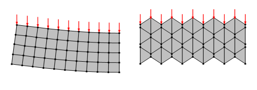
See also Reduced Integration and Hourglass Stabilization in the Structural Mechanics Theory chapter.